
Cubes were tedious to work out by hand, and Chapman printed a table of them at the end of his treatise for stability calculations. His French translator, judging it to be in daily use, checked every entry1.
Figures and tables have more room in landscape.
Chapter 2: Numerical integration for ship geometry
Version 1.0 · last revised 5 November 2026 · corrections
Prologue: Chapman’s quarter circle
In 1775 the Swedish shipbuilder Fredrik Henrik Chapman published a treatise on shipbuilding, the Tractat om Skepps-Byggeriet, which his French translator called the first work on the subject by a man of the trade1. Its first chapter is about displacement. A ship, Chapman explains, sinks until it displaces its own weight of water. If the weight of the hull and rigging is known and the displacement is known too, the weight of the cargo is their difference. For warships and privateers, whose ballast and stores were fixed, a reliable displacement allowed a designer to give a ship good stability and good sailing together. The methods in use for calculating it were, in his judgement, imperfect, and he offered another, illustrated by examples, in the hope that shipbuilders would find it simple enough to stop being daunted by the amount of arithmetic the older methods demanded1.
The usual practice, his French translator explained, joined the ends of neighbouring ordinates by straight lines; Chapman’s method treated the curve through three neighbouring ordinates as part of a parabola1. The area under each such piece is then found by geometry: the trapezium under the chord, plus two-thirds of the parallelogram that encloses the parabolic segment above it. Added up along a curve divided into an even number of equal parts, these pieces give a rule that every naval architect still learns. The first and last ordinates are multiplied by 1, the others alternately by 4 and 2, and the sum is multiplied by one-third of the spacing1.
To show that the rule was accurate enough for practice, Chapman applied it to a quarter of a circle of radius 8, whose area he could also find exactly, with five ordinates 1 apart, from the centre out to half the radius (Fig. 2.1). The rule gave 30.611312 for the area under those ordinates. Subtracting the triangle between the centre, the last ordinate and the arc left a sector of 30°, and three such sectors gave 50.2647 for the quadrant, against the exact . The calculation was, in our translation of his words, exact “to the fifth figure”; a footnote in the French edition adds that the ordinary way of calculating gave about a twentieth of a square foot less1.
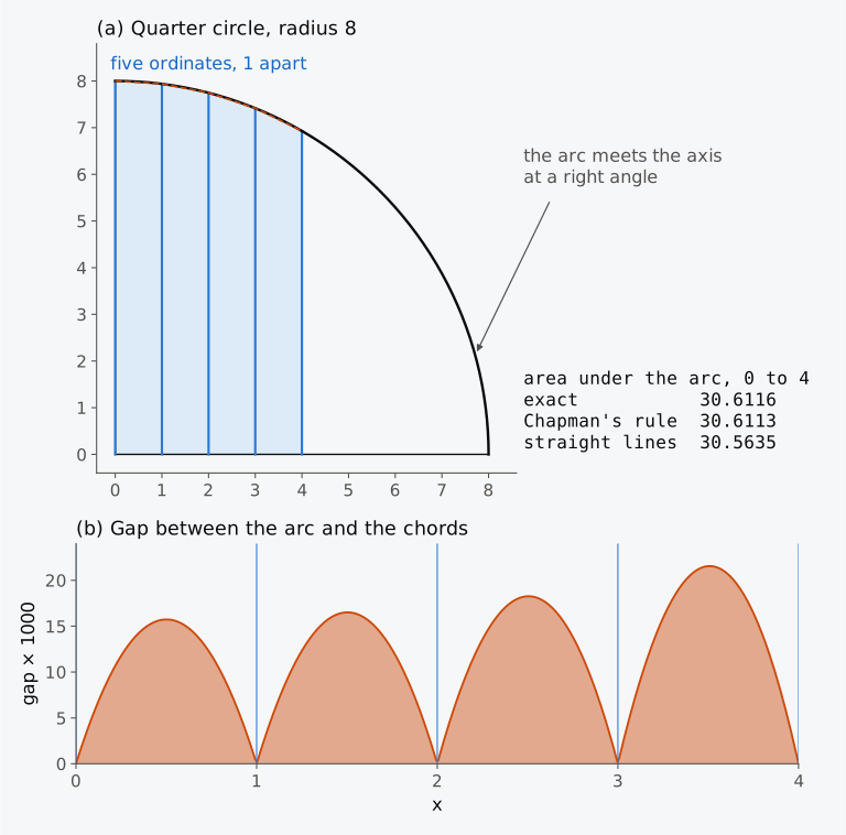
Figure 2.1 Chapman’s test of his rule: (a) a quarter circle of radius 8 with five ordinates 1 apart; (b) the gap between the arc and the straight chords, magnified 1000 times.
He then turned to a ship. For a privateer whose lines are drawn in the treatise, he measured the half-breadths of seventeen equally spaced sections at seven waterlines, 1.62 feet apart, put the seven ordinates of each section through the rule, and added the small triangle between the lowest waterline and the keel. The section areas were then treated as ordinates in their turn, 6.27 feet apart, and put through the rule again along the length, and the slivers beyond the end sections, towards the stem and the sternpost (the upright timber rising from the after end of the keel), were estimated separately. Doubled for both sides, the result was 16,210 cubic feet (about 420 to 560 m³, depending on the foot used), measured, he noted, to the outside of the frames and excluding the planking, the stem, the sternpost and the keel. In today’s terms this is a moulded volume. The moments of the section areas gave him the longitudinal position of the centre of the displacement, and, rearranging the ordinates by waterline, he found the areas of the seven waterplanes and from them its height1.
Chapman, born in 1721, was the son of the superintendent of the naval dockyard at Gothenburg, and went to England in 1750 to improve his mathematics. In London he took lessons from Thomas Simpson, who taught mathematics at the Royal Military Academy at Woolwich, and Simpson reportedly taught him this rule2. Simpson, a weaver who had taught himself mathematics, never claimed to have invented it; he acknowledged learning it from Newton3, and it had been published in 1730 by James Stirling4. After further study in France and Holland, Chapman returned to Sweden in 1757 and made it his habit to calculate the displacement of his ships, also as a function of draught, and their metacentre, with the parabolic rule2. In Britain it kept Simpson’s name, and by the end of the nineteenth century Attwood4 could describe it as the rule “most extensively used” in ship calculations. Three-quarters of a century later, the International Convention for the Safety of Life at Sea, 1974 (SOLAS), as adopted, required the cubic capacity of a lifeboat to be found by “Simpson’s (Stirling’s) Rule” or by a method of equal accuracy, and the number of persons the boat could carry was based on that capacity5.
Chapman stopped his test at half the radius. Beyond that point the arc turns down ever more steeply and meets the axis at a right angle, and the hull of a ship has places like the end of the quadrant. Where a round bilge leaves the flat bottom along an arc of a circle, the half-breadth of the section, plotted against the height above the keel, starts with a vertical tangent, as Chapman’s arc does where it meets the axis. The forefoot, where the stem curves down into the keel, and the stern turn in profile as a round bilge turns in section. A table of offsets, however, gives no ordinates between its stations from which such places could be found. We return to Chapman’s quadrant in Sec. 2.7, where the error of a rule is estimated.
In this chapter
By the end of this chapter you will be able to:
- integrate a table of offsets by the trapezoidal rule and Simpson’s rules;
- compute the centre of flotation and the transverse and longitudinal second moments of a waterplane;
- find the volume and the centre of buoyancy on a displacement sheet, and the volume curve;
- estimate the error of a result by a test case and at another spacing, and find a mistyped area from second differences.
What it assumes. You need the integrals of Eqs. (1.6) to (1.9) and the table of offsets of Sec. 1.5.3. The Wigley hull of Eq. (1.5) is the test case with exact answers.
A first reading. Sections 2.1 to 2.8 carry the main thread, from offsets to areas, moments, volumes and their error; the rules of Sec. 2.4 for real tables of offsets are used throughout Secs. 2.5 to 2.8. On a first reading Sec. 2.4.5, on the ends of a curve, and Sec. 2.5.5, on the moment of the area between two ordinates, can be skimmed, and the alternatives to Simpson’s rules in Sec. 2.9 can wait for a second reading.
2.1 From offsets to integrals
At the end of Chapter 1 you had the hull as a table of half-breadths at stations and waterlines, or as a surface that can be cut wherever you choose, and the integrals for its volume, waterplane area and centres written down but, for the Series 60 hull, not yet evaluated. Every quantity that the later chapters need is an integral of this geometry. The area of a waterplane is an integral of its half-breadth along the length; the area of a section is an integral of its half-breadth up the height; the volume is an integral of section areas along the length, or of waterplane areas up the height; and the centres and second moments are integrals of half-breadths and areas multiplied by a distance or raised to a power (Sec. 2.5). They are listed in Table 2.1, with the chapters in which each is used.
Table 2.1 The integrals of ship geometry. is the half-breadth of the waterline, the immersed section area and the waterplane area at height .
| Quantity | Integral | Integrand | Used in chapters |
|---|---|---|---|
| Waterplane area | half-breadth | 3 (tonnes per centimetre immersion), 7 | |
| Centre of flotation | 3 (small loads), 4 (longitudinal metacentre), 6 (trim), 7 | ||
| Transverse second moment | 4 (metacentric radius), 7 | ||
| Longitudinal second moment | 4 (longitudinal metacentre, moment to change trim), 6 (trim), 7 | ||
| Section area to height , | half-breadth of the section | 1 (Bonjean curves), 7 (trimmed waterlines), 12 | |
| Displacement volume | or | section or waterplane area | 3, 4, 7 |
| Centre of buoyancy , | , | , | 3, 4, 7 |
| Each quantity above, at an angle of heel | as above, over inclined waterplanes | 8 (GZ) | |
| Area under the curve of righting levers | righting lever | 9, 11 | |
| Volumes of tanks and compartments | as , over a compartment | 5, 12 | |
| Second moment of the free surface in a tank | as , about the longitudinal axis through its centroid | half-breadth of the free surface | 5 |
Every integrand in the table is known only at a finite set of points. For a lines plan they are the stations and waterlines; for a surface model, they are wherever we choose to cut it; for the righting lever of Chapter 8, they are the angles at which it has been computed. We need a rule that turns a list of ordinates at abscissae into an approximation of the integral. All the rules of this chapter take the form of a weighted sum of the ordinates,
in which the weights depend only on the positions , not on the ordinates. Written as small whole numbers with a common factor taken outside, the weights are called multipliers in naval architecture. A rule is a set of positions and weights, chosen once and applied to any curve. The products were traditionally called the functions of the ordinates, and a calculation laid out in a table of ordinates, multipliers and products is still the clearest way to see what a rule does.
There are three ways to arrive at the weights. One is geometric, as Chapman’s was: replace the curve between ordinates by simple pieces whose areas are known. A second replaces the curve by the polynomial that passes through the ordinates and integrates the polynomial exactly; this is the route that generalizes most easily, and it is used below for unequal spacing. A third expands the integrand in a Taylor series about each ordinate, which is how the error of a rule is found; all three lead to the same rules.
Two of the reference hulls of Chapter 1 serve as test cases throughout. The surface of the Wigley hull is given by a formula, so its integrals are known exactly and the error of any rule applied to its offsets can be measured. Its offsets in Table 1.2, eleven stations 10 m apart and five waterlines 1.5625 m apart, are the input. The Series 60 hull is the realistic case, and for it there is no exact answer. Its input is the table of offsets in which Todd6 published it, transcribed in Chapter 1: 25 stations, with half stations near both ends, and waterlines at the baseline and at 0.075, 0.25, 0.5, 0.75 and 1.0 times the design draught, the uneven spacing that a real table often has. Todd’s own tabulated values, and those of the surface that Chapter 1 built through Todd’s table (below called simply the smooth surface), serve for comparison with the results from the table. The three are compared in Sec. 2.6.3, and the difference from Todd’s displacement is discussed in Sec. 2.7.
2.2 The trapezoidal rule
The simplest rule, and the usual practice that Chapman set out to replace, joins the tops of neighbouring ordinates by straight lines and adds up the trapezia underneath. A strip of width between ordinates and has area , and the sum over all strips is
which for equal spacing becomes the trapezoidal rule,
Its multipliers are ½, 1, 1, …, 1, ½, because each strip gives half its width to each of its two ordinates, and every ordinate except the first and the last belongs to two strips. The rule is exact for straight lines but not, in general, for curves, and its error is the sum of the slivers between the chords and the curve (Figs. 2.1(b) and 2.2). Where the curve bulges away from the base, as a waterline does, each chord cuts inside it and the rule underestimates the area; where the curve sags towards the base, each chord passes outside it and the rule overestimates4. To first order, each sliver is the area between a chord of length and a parabola with the curvature of the curve, , and adding the slivers over the interval gives
where is the value given by the rule and is some point in the interval7. The sign agrees with the picture. Where the curve bulges away from the base, is positive and the rule is too small. An error quoted in per cent is that of the rule’s result relative to the exact value, so a rule that is too small has a negative percentage error. The value of is not known in general, and the formula is more useful for what it says about spacing. The error is proportional to , so halving the spacing reduces it to about a quarter. A rule whose error falls as is said to be of order ; the trapezoidal rule is of order 2.
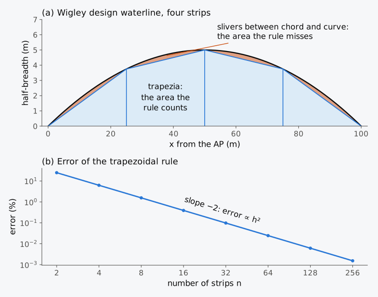
Figure 2.2 The trapezoidal rule on half of the Wigley design waterline: (a) four strips, with the slivers between chords and curve; (b) the error against the number of strips.
Example 2.1. The trapezoidal rule on the Wigley waterplane. The Wigley hull is 100 m long and 10 m wide, and the half-breadths of its design waterline at stations 0 to 10, 10 m apart, are 0, 1.8, 3.2, 4.2, 4.8, 5.0, 4.8, 4.2, 3.2, 1.8 and 0 m. Find the waterplane area by the trapezoidal rule. Compare it with the exact value , and predict the error with 20 strips instead of 10.
A second-order rule converges slowly; to bring the error of Example 2.1 down to 0.01 % would take about 100 strips, and a real table of offsets has 20 or so. The trapezoidal rule nevertheless remains in use, because it requires only that the curve be close to its chords. It works for any spacing and never overshoots between the ordinates. With the closely spaced ordinates that a computer can supply, its simplicity outweighs its low order. For some integrands the rule is much more accurate than its error formula suggests, for instance when the slope of the integrand is zero at both ends (Sec. 2.5.3).
2.3 Simpson’s first rule
Chapman’s rule replaces the chord by a parabola. His construction (Fig. 2.3) takes three equally spaced ordinates , , , a distance apart, and passes a parabola through their tops. The area under the parabola is the trapezium under the chord from to , of area , plus the parabolic segment between the chord and the curve. That segment is two-thirds of the parallelogram that encloses it, a result known since Archimedes, and the parallelogram has width and height , the amount by which the middle ordinate rises above the chord. Adding the two,
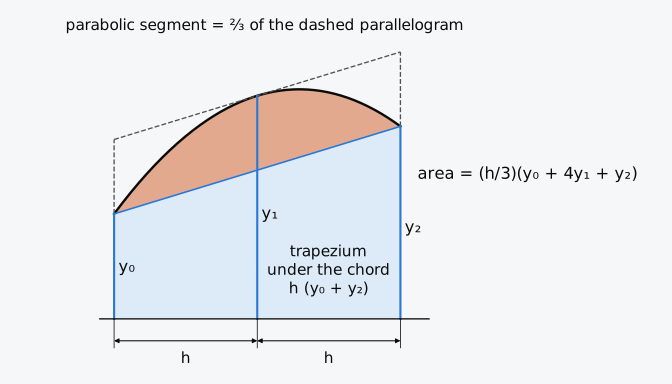
Figure 2.3 Simpson’s first rule by Chapman’s construction: the trapezium under the chord, plus two-thirds of the enclosing parallelogram.
Applied to successive pairs of strips along a curve divided into an even number of equal intervals, the rule for one pair gives Simpson’s first rule,
with multipliers 1, 4, 2, 4, …, 2, 4, 1. They are found by writing the multipliers 1, 4, 1 of each pair under its own three ordinates and adding each column4, as here for three pairs:
| Ordinate | |||||||
|---|---|---|---|---|---|---|---|
| First pair | 1 | 4 | 1 | ||||
| Second pair | 1 | 4 | 1 | ||||
| Third pair | 1 | 4 | 1 | ||||
| Multiplier | 1 | 4 | 2 | 4 | 2 | 4 | 1 |
The ordinates at the junctions of the pairs carry 2, because each belongs to two pairs; the rule needs an even number of intervals, that is, an odd number of ordinates.
The rule was built to be exact for a parabola, and symmetry makes it exact for a cubic as well. Measured from the middle ordinate, a cubic term is odd: it contributes equal and opposite amounts on either side, so its integral over the pair is zero, and the rule, whose weights are symmetric about , also gives zero for it. The first term the rule cannot integrate exactly is the quartic, and repeating the reasoning that gave the error of the trapezoidal rule, with that term, gives the error of Simpson’s rule7
(the constant is found in Exercise 2.9). Simpson’s rule is of order 4, so halving the spacing reduces the error to about one-sixteenth. With the same ordinates as the trapezoidal rule it gains two orders, at the cost of a constraint on their number, and the gain depends on the curve being smooth (Sec. 2.7).
Simpson’s rule can also be obtained from the trapezoidal rule. Let and be the trapezoidal results with spacing and with every other ordinate, spacing . Both errors are proportional to the square of the spacing, so the error of is about four times that of , and the combination cancels the leading term. Written out, the combination is Simpson’s first rule, the trapezoidal rule with its main error removed. Combining two results to cancel the leading error term works for any rule whose order is known, and gives the error estimate of Sec. 2.7.
Example 2.2. Simpson’s rule on the Wigley waterplane. The design waterline of the Wigley hull has half-breadths of 0, 1.8, 3.2, 4.2, 4.8, 5.0, 4.8, 4.2, 3.2, 1.8 and 0 m at stations 0 to 10, 10 m apart. Find the waterplane area by Simpson’s rule.
In Example 2.2 the parabolic rule gives the waterplane area exactly, where the straight-line rule of Example 2.1 is 1 % out. The volume of the Wigley hull shows the difference again, because its sections are parabolas in and its sectional-area curve is a parabola in . Simpson’s rule applied to the five waterlines of each section and then to the eleven section areas gives m³ exactly. The trapezoidal rule, applied in both directions, gives 2707.03 m³, 2.55 % low.
2.4 Adapting the rules to real tables of offsets
The Wigley offsets used so far have eleven stations at one spacing and an even number of intervals, and a real table of offsets is seldom as tidy. The ends of a ship curve more sharply than its middle, so designers add half stations there, as Todd did at stations 0.5, 1.5, 18.5 and 19.5. Near the bottom the bilge turns through a right angle within a metre or two, so the lowest waterlines are placed closer together, as Todd’s are, at the baseline and 0.075 times the draught. Nor is the number of intervals always even. Each of these cases is handled by keeping in view the idea behind Simpson’s rules, a polynomial through a few neighbouring ordinates (a parabola through each successive pair of intervals, or a cubic through three), integrated exactly. The parabola of a pair also gives the area over a single interval. A curve that ends between ordinates needs, in addition, an assumption about its shape beyond the last ordinate.
2.4.1 Half stations
Where the spacing is halved, each pair of half-intervals is a Simpson pair with spacing , so its multipliers 1, 4, 1 are halved when everything is written over the common factor . Joining the halved pattern ½, 2, 1, 2, ½ at the ends to the normal pattern 1, 4, 2, …, 4, 1 between them, and adding the multipliers where the two meet, gives the sequence for Todd’s 25 stations (Fig. 2.4(b)):
| Station | 0 | 0.5 | 1 | 1.5 | 2 | 3 | 4 | … | 16 | 17 | 18 | 18.5 | 19 | 19.5 | 20 |
|---|---|---|---|---|---|---|---|---|---|---|---|---|---|---|---|
| Halved pattern | ½ | 2 | 1 | 2 | ½ | ½ | 2 | 1 | 2 | ½ | |||||
| Normal pattern | 1 | 4 | 2 | … | 2 | 4 | 1 | ||||||||
| Multiplier | ½ | 2 | 1 | 2 | 1½ | 4 | 2 | … | 2 | 4 | 1½ | 2 | 1 | 2 | ½ |
The sum of the products is multiplied by , where is the spacing of the whole stations. Halving the multipliers wherever the interval is halved also serves for quarter stations and for the second rule below4,8. Some tables halve every multiplier, to ½, 2, 1, 2, …, with 1 and 2 instead of 2 and 4 at the whole stations, and multiply the sum by instead of . The result is unchanged, and these half multipliers save a little arithmetic8,9. They are used, for instance, in a worked calculation of displacement from section areas8.
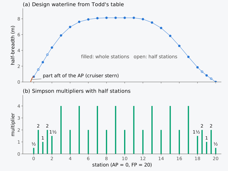
Figure 2.4 Todd’s table as input to the rules: (a) the design waterline at 25 stations; (b) Simpson multipliers with half stations at both ends.
2.4.2 Simpson’s second rule
A cubic through four equally spaced ordinates, integrated over the three intervals between them, gives Simpson’s second rule,
with composite multipliers 1, 3, 3, 2, 3, 3, 2, …, 3, 3, 1 and the factor . Its weights follow from the condition that the rule integrate 1, , and exactly. With the origin at the middle of the three intervals, the ordinates stand at and ; by symmetry the inner two carry one weight and the outer two another, , and the odd powers are then integrated exactly whatever and are. The constant and give
so that and , the weights of the second rule8. Like the first rule, it is exact for cubics and its error is of order 4. The constant of its error is in place of the of the first rule, and at a given spacing its error is about twice as large. It is used for a number of intervals that is a multiple of three, or, combined with the first rule, for any odd number of intervals: three intervals by the second rule and the rest in pairs by the first8.
2.4.3 Unequal intervals
When the two intervals of a pair are not equal, the parabola through the three ordinates can still be integrated exactly. For ordinates , , with intervals and between them, the result is
which reduces to Simpson’s rule for one pair when (Exercise 2.8). The weight of becomes negative when the second interval is more than twice the first, , and that of in the opposite case. For Todd’s lowest waterlines, at 0, 0.075 and 0.25 times the draught, , and the weight of the baseline ordinate is . The sign follows from the parabola (Fig. 2.5(a)). Raising while and stay fixed makes the parabola curve upwards more strongly. Over the long second interval it then sags below its chord, and the area lost there is more than the area gained over the short first interval. At the Series 60 draught of 6.5024 m the intervals are 0.488 m and 1.138 m, and a rise of 1 m in adds 0.219 m² under the parabola over the first interval and removes 0.310 m² over the second, a net change of −0.090 m², which is the weight of in metres. The negative weight is a property of the parabola, and it allows the rule to amplify errors in the ordinates, the more so the more unequal the intervals (Fig. 2.5(b)).
For any spacing, the intervals are paired from one end and this rule is applied to each pair; if one interval is left over, its area is taken from the parabola through the last three points. This is the construction behind the simpson function of the SciPy library10: for an odd number of equally spaced ordinates it is Simpson’s first rule, and for any other set it is the piecewise-parabolic rule just described. Version 1.18.1 was checked, and its results agree with this chapter’s scripts to rounding.
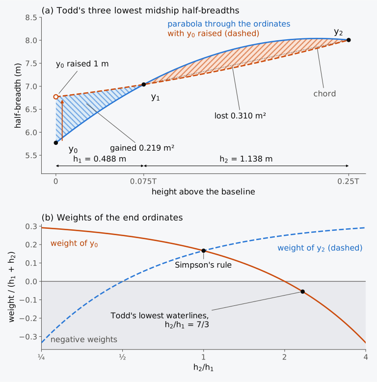
Figure 2.5 The negative weight of the rule for unequal intervals: (a) the parabola through Todd’s three lowest midship half-breadths, and with the lowest raised by 1 m (dashed); (b) the weights of the end ordinates against the ratio of the intervals.
2.4.4 The area between two ordinates
The parabola through three equally spaced ordinates can also be integrated over its first interval only, which gives the area between and :
This is the five-eight rule, sometimes called Simpson’s third rule4,11. The 5 belongs to the end ordinate of the pair that bounds the strip, the 8 to the middle ordinate and the −1 to the other end ordinate of the pair; for the other strip of the pair the order is reversed. Attwood checked it on a curve with ordinates of 8.5, 10.4 and 11.85, 2 apart: the five-eight areas of the two halves, 18.97 and 22.32 in his figures (18.975 and 22.325 before rounding), add up to the 41.3 that Simpson’s rule gives for the pair, as they must, since the two sets of weights add up to those of Simpson’s rule. With unequal intervals, the interval integrated and the next, the weights are
With the five-eight rule and its form for unequal intervals, a curve can be integrated up to an ordinate that is not at the end of a Simpson pair, as the integral with a variable upper limit requires (Sec. 2.8.1). Neither form is exact for cubics. Simpson’s rule owes its exactness for cubics to the symmetry about the middle ordinate, and that symmetry is lost when only one interval of the pair is integrated.
2.4.5 Curves ending between ordinates
A curve seldom ends at a station. The design waterline of the Series 60 hull carries on 2.06 m aft of the AP, to the cruiser stern6, and a curve of section areas taken to a low waterline may end between stations at both ends. There are four ways of including such a part, each resting on an assumption about the curve beyond the last ordinate, where the table gives nothing.
The first is to measure one extra ordinate, midway between the last station and the extremity, and to integrate the end as a Simpson pair of its own, with a zero ordinate at the extremity. Its multipliers are 1, 4 and 1 times the ratio of the half-length of the end to the station spacing, and they are added to those of the main integration where the two meet, so that one sum gives the whole area8. The US Navy’s Ship Hull Characteristics Program worked in this way: where a curve did not end at a station, it extrapolated the curve to the axis and placed one offset midway between the extremity and the first known offset8. The second is to replace the end by a shape whose area and centroid are known, a triangle or a parabola, as in Example 2.3. The third keeps the stations and changes the end ordinate instead: a reduced ordinate is chosen, by eye or by a construction, with which the rule gives the area under the real curve7. The fourth takes the shape of the end from the table itself. The extremity is taken as an ordinate of zero, and the parabola through it and the two nearest ordinates is integrated over the end by the five-eight rule for unequal intervals, Eq. (2.11). A related rule, for a curve that ends short of a station, also assumes a parabola, fixed by the two last ordinates and a fictitious, negative ordinate read at the station beyond the extremity from the curve continued past it8.
The endings that these assumptions give for the Series 60 waterline are drawn in Fig. 2.6. A parabola with its vertex at the AP leaves the AP without slope, and a parabola with its vertex at the extremity meets the centreline at a right angle. Both enclose two-thirds of the rectangle that bounds them, so each has an area of 1.83 m² for the two sides together, but their centroids lie at 3/8 and at 0.4 of the length of the end aft of the AP. The smooth surface carries the waterline almost straight from the AP to the extremity and encloses 1.39 m². The three curves cross the extra ordinate at 0.500 m, 0.471 m and 0.340 m. With these midway ordinates, Simpson’s rule on the extra pair gives 1.83 m² for the parabola with its vertex at the AP, which it integrates exactly, and 1.39 m² for the surface. For the parabola with its vertex at the extremity it gives 1.75 m², because that curve meets the centreline with a vertical tangent, as Chapman’s arc meets its axis, and the parabola of the rule cannot follow it. In the fourth way the ordinates are 0 at the extremity, 0.666 m at the AP, 2.06 m forward of it, and 1.569 m at station ½, a further 3.048 m forward. Equation (2.11) gives 0.694 m² for one side and 1.39 m² for both, and the first moment of the parabola puts its centroid 0.335 of the length of the end aft of the AP. These are the values of the surface’s ending to the precision printed. Both curves pass through the three points, and between them they hardly differ: the parabola crosses the extra ordinate at 0.339 m, against 0.340 m for the surface, and Fig. 2.6 does not draw it separately. The ordinate at the AP and the length of the end are known, but the shape between them is not, and the possible endings differ in area by about a quarter of the area of the end. That is 0.03 % of the waterplane; its effect on the centre of flotation is found in Example 2.5.
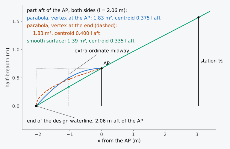
Figure 2.6 Three possible endings of the Series 60 design waterline aft of the AP, with the extra ordinate midway between the AP and the end of the waterline.
A volume also has ends beyond its ordinates, the part below the lowest waterline, where the keel rises aft or the hull narrows to a fin, and the parts beyond the end stations. Chapman allowed for both on his privateer, with the small triangle below the lowest waterline in each section and a separate estimate of the slivers beyond the end sections. Such parts are computed separately, each with its volume and centre, and combined with the main body by moments, as in Attwood’s worked calculation of displacement for the appendage below its lowest waterplane4. The volume of the shell and of true appendages, which lie outside the moulded surface, is also added separately (Sec. 3.4.6).
Table 2.2 Waterplane sheet for the design waterline of the Series 60 hull, from Todd’s offsets: the area. is the half-breadth (m), printed to 1 mm; products are computed from the unrounded half-breadths. The multipliers are those of Fig. 2.4(b).
| Station | (m) | (m) | Multiplier | Product for area |
|---|---|---|---|---|
| 0 | 0.00 | 0.666 | ½ | 0.333 |
| 0.5 | 3.05 | 1.569 | 2 | 3.137 |
| 1 | 6.10 | 2.503 | 1 | 2.503 |
| 1.5 | 9.14 | 3.454 | 2 | 6.909 |
| 2 | 12.19 | 4.357 | 1½ | 6.535 |
| 3 | 18.29 | 5.893 | 4 | 23.571 |
| 4 | 24.38 | 6.966 | 2 | 13.931 |
| 5 | 30.48 | 7.616 | 4 | 30.464 |
| 6 | 36.58 | 7.925 | 2 | 15.850 |
| 7 | 42.67 | 8.079 | 4 | 32.317 |
| 8 | 48.77 | 8.128 | 2 | 16.256 |
| 9 | 54.86 | 8.128 | 4 | 32.512 |
| 10 | 60.96 | 8.128 | 2 | 16.256 |
| 11 | 67.06 | 8.128 | 4 | 32.512 |
| 12 | 73.15 | 7.957 | 2 | 15.915 |
| 13 | 79.25 | 7.527 | 4 | 30.106 |
| 14 | 85.34 | 6.836 | 2 | 13.671 |
| 15 | 91.44 | 5.836 | 4 | 23.344 |
| 16 | 97.54 | 4.568 | 2 | 9.136 |
| 17 | 103.63 | 3.178 | 4 | 12.712 |
| 18 | 109.73 | 1.853 | 1½ | 2.780 |
| 18.5 | 112.78 | 1.300 | 2 | 2.601 |
| 19 | 115.82 | 0.829 | 1 | 0.829 |
| 19.5 | 118.87 | 0.415 | 2 | 0.829 |
| 20 | 121.92 | 0.000 | ½ | 0.000 |
| Sum | 345.01 |
Example 2.3. The waterplane of the Series 60 hull from Todd’s table. Using the half-breadths of the design waterline at Todd’s 25 stations (Table 2.2), find the waterplane area by Simpson’s rule with half stations, add the small part of the waterplane aft of the AP, where the waterline ends 2.06 m behind it, and find . The hull has = 121.92 m and = 16.256 m.
2.5 Moments, centroids and second moments
The area of the Series 60 waterplane came from 25 half-breadths and their multipliers in Table 2.2. Its centre of flotation needs one more column on the waterplane sheet, because a centre is a first moment divided by an area, and a first moment is the integral for an area with the integrand multiplied by a distance. The rule that gave the area therefore serves for the moment, applied to the products instead of . In a hand calculation the distance is written as a lever in units of the station spacing, here the station number , with , and the factor is applied once at the end:
where are the multipliers. Any reference point for the levers will do, provided that all the products of one moment use it. Levers measured from amidships, positive forward and negative aft, keep the numbers small and were the traditional choice4. In this section the first moment is taken about the AP, the origin of every longitudinal position, and its levers are the station numbers; the second moment is taken about the transverse axis amidships, where the squares of the levers are smaller.
2.5.1 Moments of a strip and the transverse second moment
The integrands come from the moments of a strip (Fig. 2.7(a)). A strip of the waterplane, of width and half-breadth on one side, has area , and all of it lies at the distance from the AP, so its first and second moments about the AP are and . About the centreline the distance varies across the strip, from 0 at the centreline to at the waterline. The centroid of the strip is at , which gives its first moment about the centreline, . For any plane area whose ordinates stand on a straight base, the integrand gives the moment about that base (Exercise 2.6). The second moment of the strip about the centreline adds up the squares of the distances of its elements ,
and for both sides of the waterplane it gives the transverse second moment of the waterplane, about the centreline8,9,
It is called transverse because it governs heel, the inclination of the ship in the transverse plane. How far the centre of buoyancy moves sideways when the ship heels by a small angle depends on and on the volume, and that movement fixes the position of the metacentre. Second moments of area are also called moments of inertia, and is the transverse moment of inertia of the waterplane12. It depends only on the geometry of the waterplane and is measured in m⁴. The mass moment of inertia of the ship in roll is a different quantity12, the mass of the ship times the square of its radius of gyration about a longitudinal axis through its centre of gravity, measured in t·m². The integrand of is the cube of the half-breadth, so the breadth of the waterplane dominates its value.
Historical note: Chapman’s table of cubes
The transverse inertia coefficient compares with , the second moment of the rectangle about its centreline12,13,
which is 1 for a rectangle, 48/105 = 0.457 for the Wigley waterplane (Example 2.4) and 0.544 for the Series 60 waterplane (Example 2.5). The second moment of the rectangle overstates by the factor , 2.19 for the Wigley waterplane and 1.84 for the Series 60, and is no substitute for integrating the cubes of the half-breadths.
2.5.2 The longitudinal second moment
The longitudinal second moment is the second moment of the waterplane about the transverse axis through its centre of flotation F. It is taken first about a convenient transverse axis, through the AP or amidships, and then moved to F (Fig. 2.7(b)). Writing each distance from the AP as and squaring it,
The middle integral is the first moment of the waterplane about an axis through its own centroid, which is zero by the definition of the centroid, and the last term is . What remains is the parallel-axis theorem,
The second moment about an axis through the centroid is the smallest of all those about parallel axes: moving the axis a distance away from the centroid adds , where is the area, and moving it back to the centroid subtracts it8,14. A sign error here is easy to make and hard to see, because both results look plausible.
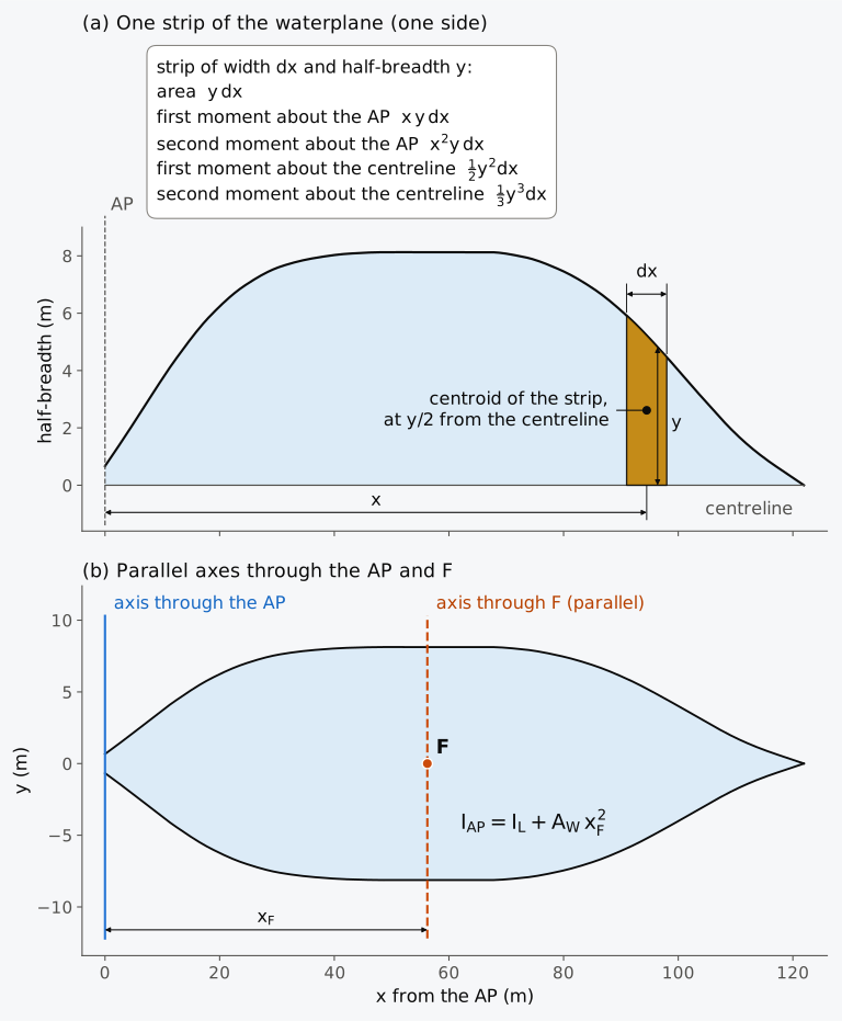
Figure 2.7 Moments of the Series 60 design waterplane: (a) one strip; (b) parallel axes through the AP and through the centre of flotation F. Half-breadths are drawn at 5 times (a) and 2.5 times (b) the scale of lengths.
The longitudinal second moment governs trim, the inclination of the ship in the longitudinal plane, and it is taken about F because a ship at constant displacement trims about F. Only about an axis through the centroid of the waterplane are the wedges immersed and emerged in a small trim equal in volume9. The longitudinal inertia coefficient compares with , the second moment of the rectangle about its transverse axis through the centre12,
The design waterline of the Wigley hull is with , and its centre of flotation is amidships, so that
and = 0.4; the Series 60 waterplane has = 0.428 (Example 2.5).
The two second moments take their value from different parts of the waterplane. In each strip is weighted by the square of its distance from F, and in by the square of its own half-breadth. The quarters of the length at the two ends of the Wigley waterplane, where , hold 5/16 of its area but give 47/64 of , about 73 %, and only 289/2048 of , about 14 %:
Errors in the end offsets, half stations included, and in the shape assumed aft of the AP matter far more for than for .
Second moments about other axes are built from strips and moved by the parallel-axis theorem. A waterplane that is not symmetric about the centreline, as at an angle of heel or with one side damaged, also has a product of inertia, and its principal axes are no longer the centreline and a transverse line14. The heeled waterplanes of Chapter 8 and the damaged waterplanes of Chapter 12 are asymmetric in this way. The product of inertia of a polygon is given in Sec. 2.9.3.
2.5.3 Accuracy of the rules for second moments
A rule that is exact for the half-breadth need not be exact for its cube, the integrand of , or for , the integrand of the second moment about a transverse axis. The accuracy of matters because in Chapter 4 it is divided by the volume to give the distance through which the centre of buoyancy moves sideways per radian of a small heel, and a relative error in passes unchanged into that distance.
Example 2.4. The transverse second moment of the Wigley waterplane. The design waterline of the Wigley hull, 100 m long and 10 m wide, has half-breadths of 0, 1.8, 3.2, 4.2, 4.8, 5.0, 4.8, 4.2, 3.2, 1.8 and 0 m at stations 0 to 10, 10 m apart. Find of the waterplane by Simpson’s rule and by the trapezoidal rule, and compare both with the exact value. Find .
Simpson’s rule integrated the parabolic Wigley waterline exactly, but the cube of the half-breadth has degree 6 and has degree 4. With ten intervals its error is −0.087 % in and −0.16 % in about amidships; Hamlin warns of such errors in general terms8. The order of a rule is also an incomplete guide to its accuracy. The error of the trapezoidal rule can be expanded as a series, the Euler–Maclaurin formula15, in which the term in is proportional to the difference of the slopes of the integrand at the two ends, , and the next term, , to the difference of the third derivatives. The cube of a half-breadth that falls to zero at both ends has zero slope there, because , so the term vanishes. The trapezoidal rule then behaves as a rule of order 4, with an error a quarter of Simpson’s and of the opposite sign; in Example 2.4 the trapezoidal rule is 0.88 m⁴ high and Simpson’s rule 3.30 m⁴ low. The effect occurs on fine waterlines with pointed ends and disappears for a waterline that ends in a transom, where is not zero.
2.5.4 The Series 60 waterplane
For the Series 60 waterplane the moments are added to the sheet of Table 2.2 as further columns, in Table 2.3.
Table 2.3 Waterplane sheet for the design waterline of the Series 60 hull, continued from Table 2.2: the moments. The lever for the moment is the station number (each lever times is the distance forward of the AP), and the product for the moment is the product for area times . The product for about amidships is the product for area times , the square of the lever from amidships, and the product for is the multiplier times . As in Table 2.2, products and sums are computed from the unrounded half-breadths; sums formed from the printed entries, or from the rounded half-breadths, differ by less than 0.003 %, which leaves the results of Example 2.5 for , and unchanged at the precision given there.
| Station | Product for area | Product for moment | Product for about amidships | (m³) | Product for |
|---|---|---|---|---|---|
| 0 | 0.333 | 0.000 | 33.32 | 0.30 | 0.15 |
| 0.5 | 3.137 | 1.569 | 283.15 | 3.86 | 7.72 |
| 1 | 2.503 | 2.503 | 202.78 | 15.69 | 15.69 |
| 1.5 | 6.909 | 10.363 | 499.16 | 41.22 | 82.44 |
| 2 | 6.535 | 13.070 | 418.23 | 82.69 | 124.03 |
| 3 | 23.571 | 70.714 | 1154.99 | 204.63 | 818.51 |
| 4 | 13.931 | 55.726 | 501.53 | 337.98 | 675.96 |
| 5 | 30.464 | 152.319 | 761.59 | 441.74 | 1766.97 |
| 6 | 15.850 | 95.098 | 253.59 | 497.70 | 995.39 |
| 7 | 32.317 | 226.218 | 290.85 | 527.36 | 2109.45 |
| 8 | 16.256 | 130.048 | 65.02 | 536.97 | 1073.94 |
| 9 | 32.512 | 292.608 | 32.51 | 536.97 | 2147.89 |
| 10 | 16.256 | 162.560 | 0.00 | 536.97 | 1073.94 |
| 11 | 32.512 | 357.632 | 32.51 | 536.97 | 2147.89 |
| 12 | 15.915 | 190.975 | 63.66 | 503.85 | 1007.70 |
| 13 | 30.106 | 391.379 | 270.96 | 426.37 | 1705.47 |
| 14 | 13.671 | 191.398 | 218.74 | 319.40 | 638.81 |
| 15 | 23.344 | 350.154 | 583.59 | 198.76 | 795.03 |
| 16 | 9.136 | 146.174 | 328.89 | 95.31 | 190.63 |
| 17 | 12.712 | 216.107 | 622.90 | 32.10 | 128.39 |
| 18 | 2.780 | 50.036 | 177.91 | 6.36 | 9.55 |
| 18.5 | 2.601 | 48.118 | 187.92 | 2.20 | 4.40 |
| 19 | 0.829 | 15.752 | 67.15 | 0.57 | 0.57 |
| 19.5 | 0.829 | 16.167 | 74.82 | 0.07 | 0.14 |
| 20 | 0.000 | 0.000 | 0.00 | 0.00 | 0.00 |
| Sum | 345.01 | 3186.69 | 7125.79 | 17520.67 |
Example 2.5. Centre of flotation and second moments of the Series 60 waterplane. From Tables 2.2 and 2.3, find the centre of flotation, and , and about the centre of flotation and . The stations are 6.096 m apart, = 121.92 m and = 16.256 m. The waterplane area is 1402.12 m² between the perpendiculars and 1403.95 m² with the part aft of the AP, which has an area of 1.83 m² and ends 2.06 m aft of the AP. Take the centroid of that part three-eighths of its length from the AP, and neglect its second moments about its own axes.
2.5.5 The moment of the area between two ordinates
The first moment of a single strip was a familiar source of error in hand calculation. The five-eight rule gives the area between two ordinates, but multiplying its three products by their levers does not give the moment of that area, because the parabola was integrated over only part of its length. The correct moment about of the area between and comes from integrating times the parabola through the three ordinates over the first interval,
the three-ten rule. Attwood4 showed the error with a curve whose ordinates are 10, 9 and 7, 4 apart: weighting the five-eight products by levers puts the centroid 2.02 from the end ordinate, when the shape of the curve requires slightly less than 2, and the three-ten rule gives 1.965.
2.5.6 An integration sheet, and a waterplane of your own (Calculator 2.1, Explorer 2.1)
Calculator 2.1 sets out the integration of a plane area as a sheet, in the form of Tables 2.2 and 2.3: for each ordinate, the weight of the rule and the products that give the area, the first moment, the second moment and, for a waterplane, the cubes of the half-breadths. The rule is Simpson’s first rule when the ordinates are equally spaced and their number is odd, and otherwise the piecewise-parabolic rule; the trapezoidal rule is shown beside it for comparison. Below the sheet, the working gives the area, the centroid, the second moments and the moment of the area about the centreline or the base.
The calculator walks through the sheets of the worked examples, for the Wigley and Series 60 design waterlines, the waterplane of Exercise 2.5 and Todd’s midship section. The ordinates of each are fixed, so that the working can be followed line by line against the example. It checks each result against what any area whose ordinates are not negative must satisfy: a positive area, a centroid between the first and the last ordinate, and second moments that are not negative. When a result fails these checks, the spacing is too uneven for the rule, as in the problem “Very uneven spacing”, and the calculator says so instead of reporting the number as a property of the area. Passing the checks does not show that a result is accurate; its error has to be estimated separately (Sec. 2.7).
Explorer 2.1 is a waterplane to build: its length, the number of ordinates and each half-breadth are set by hand, the shape is drawn as the rule sees it, through the parabola of each pair of intervals, and the sheet, the area, the centre of flotation, the second moments and the coefficients change with it. It opens on the Wigley waterline of Example 2.2, so the first area shown is 666.67 m². Where the ordinates change sharply, a parabola can dip below zero between them or rise above the largest ordinate, and the Explorer reports it. It gives no results for a waterline that crosses the centreline, and it takes the breadth from the widest point of the drawn curve.
2.6 Volumes by integrating twice
The volume was written in Chapter 1 in two ways, as an integral of section areas along the length and as an integral of waterplane areas up the height. Either way needs two integrations, taken in one of the two orders of Fig. 2.8. In the first, each section is integrated up to the waterline to give its area . Plotted against , these areas form the sectional-area curve: the area under it is the displacement volume, and the -coordinate of its centroid is the longitudinal centre of buoyancy , so integrating the curve along the length, with and without the lever , gives both. In the second, each waterline is integrated along the length to give the waterplane area , and these areas are integrated up the height. The area between the curve of waterplane areas and the height axis is again the volume, and the height of its centroid is . Chapman used both, the first for the volume and its longitudinal centre, the second for its vertical centre.
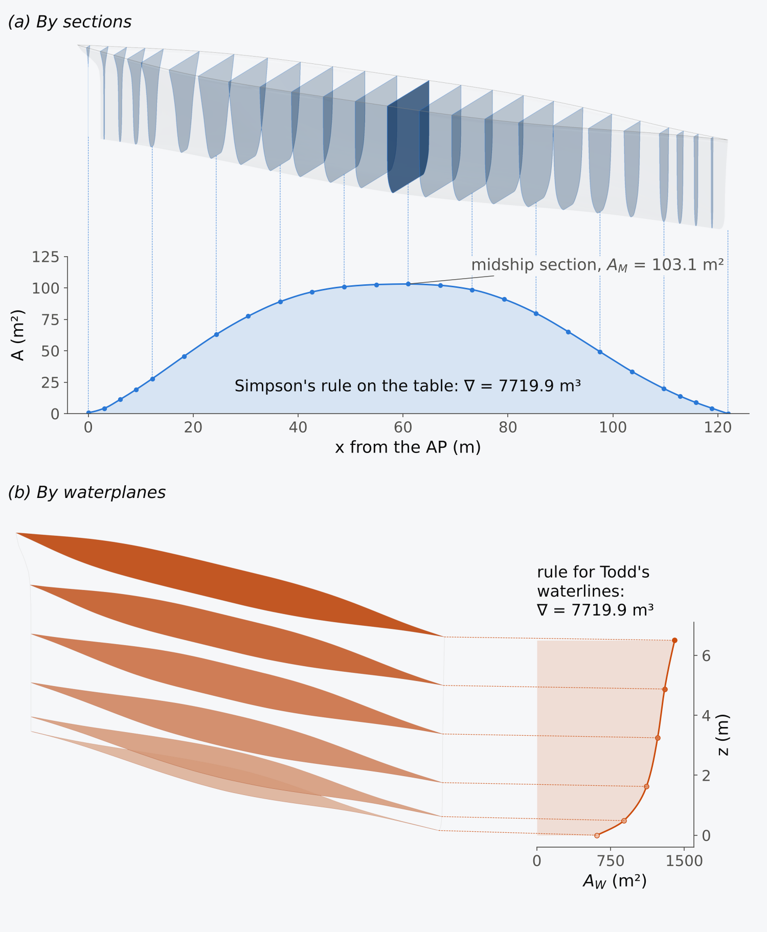
Figure 2.8 Two routes from Todd’s table to the displacement volume of the Series 60 hull: (a) by sections; (b) by waterplanes. Points are areas from the table, curves smooth guides through them. Heights are drawn 2.5 times (a) and 9 times (b) as large as lengths.
2.6.1 The displacement sheet
When both integrations were done by hand, they were set out together on one large form, the displacement sheet4,8. Its rows are the stations and its columns the waterlines (Fig. 2.9), and every offset of the table is entered once. Each row is multiplied, ordinate by ordinate, by the multipliers of the rule up the height and summed, to give a function of the area of that section. Each column is multiplied by the multipliers along the length and summed, to give a function of the area of that waterplane. The functions of the section areas, multiplied by the multipliers along the length, and the functions of the waterplane areas, multiplied by those up the height, must give equal grand totals, and this equality checks the arithmetic of the sheet. Levers in the margins give the moments: station numbers for the longitudinal centre of buoyancy and waterline numbers for the vertical centre.
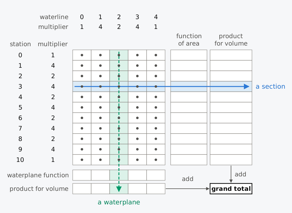
Figure 2.9 The layout of a displacement sheet for eleven stations and five waterlines, with Simpson’s multipliers. Each square is one offset; one section (solid arrow) and one waterplane (dashed arrow) are followed to the grand total.
For the Wigley hull the sheet is set out in Table 2.4. Its sections are parabolas in and its waterlines parabolas in , so Simpson’s rule is exact in both directions and every entry can be checked against the formula of the hull. The displacement sheet of the Series 60 hull, from Todd’s table and with the weights of the next subsection up the height, is given with the chapter’s data (Notes on the data).
Table 2.4 Displacement sheet for the Wigley hull. The half-breadths are in metres; the column headings give the height of each waterline above the keel and its multiplier. The station multipliers are Simpson’s, with = 10 m, and the waterline multipliers Simpson’s, with = 1.5625 m. The lever for the moment along the length is the station number; up the height it is the waterline number, 0 to 4 from the keel or 4 to 0 from the waterline.
| Station | Multiplier | 0 m (×1) |
1.5625 m (×4) |
3.125 m (×2) |
4.6875 m (×4) |
6.25 m (×1) |
Function of area | Product for volume | Product for moment |
|---|---|---|---|---|---|---|---|---|---|
| 0 | 1 | 0 | 0 | 0 | 0 | 0 | 0.0 | 0.0 | 0.0 |
| 1 | 4 | 0 | 0.7875 | 1.3500 | 1.6875 | 1.8000 | 14.4 | 57.6 | 57.6 |
| 2 | 2 | 0 | 1.4000 | 2.4000 | 3.0000 | 3.2000 | 25.6 | 51.2 | 102.4 |
| 3 | 4 | 0 | 1.8375 | 3.1500 | 3.9375 | 4.2000 | 33.6 | 134.4 | 403.2 |
| 4 | 2 | 0 | 2.1000 | 3.6000 | 4.5000 | 4.8000 | 38.4 | 76.8 | 307.2 |
| 5 | 4 | 0 | 2.1875 | 3.7500 | 4.6875 | 5.0000 | 40.0 | 160.0 | 800.0 |
| 6 | 2 | 0 | 2.1000 | 3.6000 | 4.5000 | 4.8000 | 38.4 | 76.8 | 460.8 |
| 7 | 4 | 0 | 1.8375 | 3.1500 | 3.9375 | 4.2000 | 33.6 | 134.4 | 940.8 |
| 8 | 2 | 0 | 1.4000 | 2.4000 | 3.0000 | 3.2000 | 25.6 | 51.2 | 409.6 |
| 9 | 4 | 0 | 0.7875 | 1.3500 | 1.6875 | 1.8000 | 14.4 | 57.6 | 518.4 |
| 10 | 1 | 0 | 0 | 0 | 0 | 0 | 0.0 | 0.0 | 0.0 |
| Sum | 800.0 | 4000.0 | |||||||
| Waterplane function | 0 | 43.75 | 75.00 | 93.75 | 100.00 | ||||
| Product for volume | 0 | 175.0 | 150.0 | 375.0 | 100.0 | 800.0 | |||
| Product, lever from keel | 0 | 175.0 | 300.0 | 1125.0 | 400.0 | 2000.0 | |||
| Product, lever from waterline | 0 | 525.0 | 300.0 | 375.0 | 0 | 1200.0 |
Example 2.6. The displacement sheet of the Wigley hull. The Wigley hull is 100 m long and 10 m wide and floats at a draught of 6.25 m. From Table 2.4, find the displacement volume by sections and by waterplanes, the longitudinal centre of buoyancy, and the height of the centre of buoyancy above the keel, with a check by moments about the waterline. Compare with the exact values , and .
2.6.2 Sections with uneven waterlines
Todd’s waterlines are at 0, 0.075, 0.25, 0.5, 0.75 and 1.0 times the design draught: five intervals, the first two unequal. A suitable rule for them combines two of the rules above. The first two intervals, 0 to 0.075 and 0.075 to 0.25 of the draught, form a pair for the rule for unequal intervals; the remaining three, of 0.25 each, are a case for Simpson’s second rule. In metres, for m, the weights of the six ordinates are −0.0903, 1.2902, 1.0354, 1.8288, 1.8288 and 0.6096 (Fig. 2.10(a)); they add up to the draught, as the weights of any rule must add up to the length of the interval, since the rule has to integrate a constant exactly.
Amidships the half-breadths are 5.771 m at the baseline (the half-width of the flat bottom, or flat of keel), 7.039 m at 0.075 and 8.006 m at 0.25, and 8.128 m, the full half-breadth, above. The rule gives a half-area of 51.53 m², so m² and . What the rule assumes between the ordinates is drawn in Fig. 2.10(b). Above half the draught the section is wall-sided (its side is vertical), and the rule integrates that part exactly. Below half the draught lies the whole turn of the bilge, where the half-breadth grows from 5.77 m to 8.13 m. The table gives four ordinates there, three of them up to a quarter of the draught, and the area depends on the curves that the rule draws through them: a parabola through the lowest three and a cubic from a quarter of the draught upwards.
The rule is also least reliable at the bilge. A round bilge leaves the flat of keel along an arc of a circle. Measured upwards from the keel, the half-breadth grows at first as the square root of the height, as the ordinate of Chapman’s arc does with the distance from the end of the quadrant, and no parabola can follow it. Todd gives the bilge radius as m. If all six ordinates are taken from a circular bilge of that radius, whose section has an exact area of 103.32 m², the rule gives 103.52 m², 0.19 % too much, and the trapezoidal rule 102.74 m², 0.56 % too little. The table adds an uncertainty of its own. The circle passes 0.075 at 7.208 m, where the table gives 7.039 m, and the ordinates give no means of deciding which is correct. Both effects amount to a few tenths of a per cent of the section area.
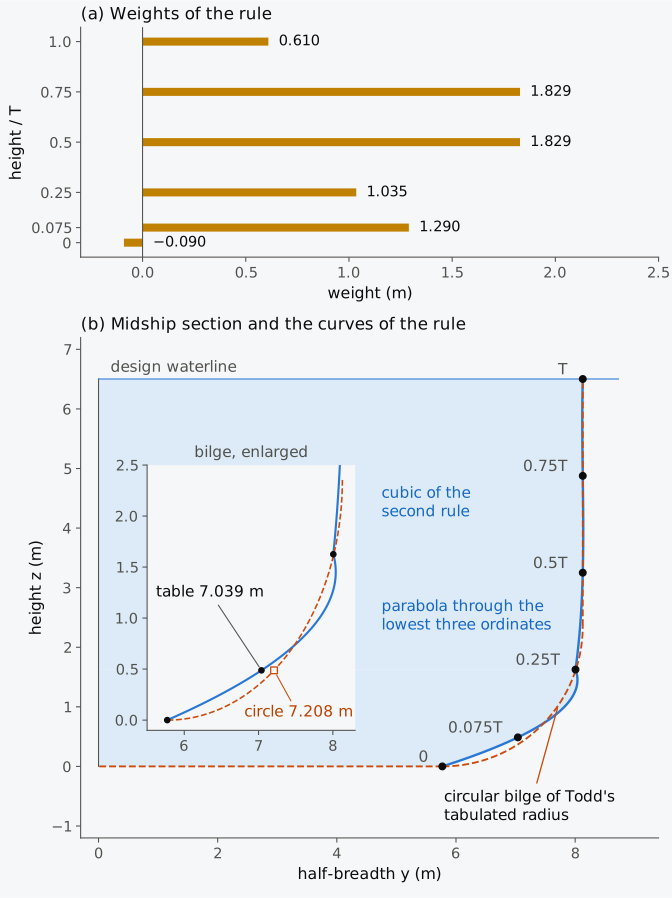
Figure 2.10 The rule for Todd’s waterlines: (a) the weights of the six ordinates; (b) the curves it draws through the midship ordinates of the Series 60 hull, with the circular bilge of Todd’s tabulated radius (dashed).
2.6.3 The volume, both ways
Applying the rule for Todd’s waterlines at all 25 stations gives the sectional-area curve, which agrees with Todd’s tabulated area fractions to within 0.004 of at every station. Integrated along the length with Simpson’s multipliers, half stations included, it gives m³. By the other route, the six waterplane areas from the baseline to the design waterline are 610.02, 885.48, 1115.05, 1228.47, 1299.65 and 1402.12 m² between the perpendiculars, and integrating them up the height with the rule for Todd’s waterlines also gives 7719.9 m³.
That the two routes agree should not be taken as a check of accuracy. Both use every ordinate of the table, each multiplied by a weight in and a weight in ; the volume is the double sum , and the order of summation does not change it. The agreement checks the arithmetic, and that was its use when the arithmetic was done by hand8,9; it does not show whether the rules suit the hull. The comparison of the two routes becomes informative only when they use different information, for instance when the ends beyond the end stations are added in one route and not in the other. The cruiser stern adds a part of the volume aft of the AP, above about 0.9, that is in neither sum; the smooth surface puts it at 0.42 m³, which is negligible.
Nor does the agreement show whether the offsets are right. An offset misread from the drawing or mistyped enters both routes alike and leaves the totals in agreement. Such an error shows instead as a point off a fair curve when the section areas or the waterplane areas are plotted4,8. Where the values are equally spaced, it also shows in their second differences, the differences between successive differences, as one value out of line, with its neighbours moved half as far the other way.
Taken with levers, the sums of the two routes give the centre of buoyancy: m, 1.47 % of the length aft of amidships, and m.
A third route to uses the vertical moment of each section area about the base, up to the waterline; integrating these moments along the length gives . With Simpson’s multipliers along the length and the rule for Todd’s waterlines up the height, it is again the double sum of the table, now with the lever as well, and it also gives 3.48 m. This route is useful because each section is integrated up to the point where the waterline cuts it. It works equally for a waterline that is not parallel to the base, when the ship is trimmed, and for a ship flooded over part of its length8 (Chapters 7 and 12).
Todd’s values and those of the smooth surface complete the comparison:
| Quantity | Todd’s table, this section | Smooth surface | Todd6 |
|---|---|---|---|
| (m³) | 7719.9 | 7709.1 | 7737.4 |
| 0.599 | 0.598 | 0.60 | |
| , aft of amidships | 1.47 % of | 1.49 % of | 1.5 % of |
| (m) | 3.48 | 3.49 |
Example 2.7. Midship section and displacement from Todd’s table. The Series 60 hull has = 121.92 m, = 16.256 m and a design draught = 6.5024 m. (a) At Todd’s six waterlines, from the baseline to the design waterline, the half-breadths of the midship section are 5.771, 7.039, 8.006, 8.128, 8.128 and 8.128 m, and the weights of the rule for these waterlines are −0.0903, 1.2902, 1.0354, 1.8288, 1.8288 and 0.6096 m. Find the area of the midship section and its . (b) The sum of the products of the 25 section areas and their multipliers, with stations 6.096 m apart, is 3799.18 m². Find , and the displacement mass in sea water.
2.7 Estimating the error
For the Wigley hull the error of every result so far could be read off against the exact value. For the Series 60 results there is no exact value, and the error has to be estimated. The error formulae of the trapezoidal rule and Simpson’s rule show how an error changes with the spacing, but not how large it is, because the derivatives they contain are not known. In practice the error is assessed by separate checks, each catching a different source of error. The error that arises where the table does not define the hull closely enough cannot be revealed by comparing rules and needs a check of its own.
Whether the rules have been applied correctly is settled by a test case with a known answer. The Wigley hull is such a case; a scheme that does not return and from its offsets by Simpson’s rule is wrong. The size of the rule’s error for a given hull and spacing is estimated by repeating the calculation with a different spacing. If and are results with spacing and from a rule of order , their errors are in the ratio , and eliminating the error between them gives an estimate both of the error and of a better value,
This is Richardson extrapolation, and for the trapezoidal rule () it is the combination that gave Simpson’s rule. For Simpson’s rule () the correction is one-fifteenth of the difference between the two results.
On Todd’s table the test can be made by dropping stations. With the eleven even-numbered stations, spacing , Simpson’s rule gives = 7729.6 m³; with all 21 whole stations, 7722.2 m³; with the half stations as well, 7719.9 m³. By Richardson extrapolation, the error of the 21-station result is about m³, which would put the integral at 7721.7 m³. The half stations give 7719.9 m³, 2.3 m³ below the 21-station result and 1.8 m³ below the extrapolated value. They add information near the ends, where the sectional-area curve changes too quickly for its error to fall as at this spacing, and the halving test cannot detect that part of the error. The error of the integration along the length is estimated at a few hundredths of a per cent. The integration up the height is less certain: replacing the second rule on the upper three intervals by parabolas through pairs, with the last interval taken from the parabola through the last three ordinates, which is equally a rule of order 4, changes to 7724.9 m³, a difference of 0.06 %. Replacing the rules of order 4 by the trapezoidal rule in one direction or in both shows which direction carries the error:
| Along the length | Up the height | (m³) | Difference from 7719.9 (m³) |
|---|---|---|---|
| Simpson’s rule, half stations included | rule for Todd’s waterlines | 7719.9 | 0 |
| Simpson’s rule, half stations included | trapezoidal rule | 7658.5 | −61.4 |
| trapezoidal rule | rule for Todd’s waterlines | 7708.4 | −11.5 |
| trapezoidal rule | trapezoidal rule | 7646.9 | −73.0 |
The trapezoidal rule in both directions is nearly 1 % low, and most of that comes from the vertical integration, where the straight lines cut the corner at the bilge. Todd’s own displacement, from his faired lines, is 7737.4 m³, 0.23 % above our result. That difference is of the order of the two effects found at the bilge, the rule’s error where the half-breadth grows as the square root of the height and the table’s own uncertainty there. Between them they account for most of it. With a rule of order 4 and stations as close as Todd’s, the accuracy of the volume is limited by the bilge rather than by the integration along the length.
The error of a good integration is small beside the other uncertainties of a displacement. The density of sea water varies with temperature and salinity, and the 1025 kg/m³ used in design is a convention7; the moulded volume differs from the true displacement by the shell and appendages, typically by 0.5 % to 1 %. A ship may also carry a stability instrument, an approved onboard computer that calculates the ship’s hydrostatics and stability for the loading carried. When such an instrument computes from a model of the hull, the IMO Guidelines for the approval of stability instruments, MSC.1/Circ.1229, accept a displacement that differs by up to 2 % from the ship’s approved data16 (Sec. 2.10.2). An error of 0.01 % from an integration rule is negligible on either scale, and an error of about 1 %, such as the trapezoidal rule made on Todd’s table, would be within that tolerance. It is not small in other terms: 1 % of the Series 60 volume is 77 m³, or 5.5 cm of mean draught, a large amount in a lightweight survey or an inclining experiment (Chapter 10).
Richardson extrapolation assumes that the error falls as , and the assumption should be checked, for instance on Chapman’s quadrant of the prologue. On his five ordinates, 1 apart from the centre to half the radius, Simpson’s rule missed the exact area, 30.6116, by 0.00025, less than a thousandth of a per cent. Had he carried ordinates 1 apart to the end of the quadrant, where the arc meets the axis at a right angle, nine ordinates would have given 49.939 against the exact 50.265, an error of 0.65 %, nearly eight hundred times the relative error of his own test. Over half the radius Chapman’s curve is smooth and Simpson’s rule converges as ; over the whole quadrant every derivative of the integrand is unbounded at the end of the arc, and the error falls only as (Fig. 2.11). With ordinates 4, 2 and 1 apart, Simpson’s rule gives 47.617, 49.338 and 49.939 for the quadrant. Extrapolating the last two with gives 49.979, still 0.57 % low, and the estimate of the error is too small by a factor of eight. The order can be found from the three results. The ratio of successive differences, , is with , and extrapolating with that order gives 50.262, within 0.006 %. Three results at halving spacings allow the assumption to be tested before it is used; two results do not.
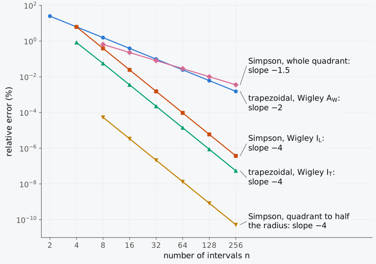
Figure 2.11 How the error falls as the spacing is reduced, for five pairs of rule and integrand. The slope of each line is the order of the rule for that integrand.
Explorer 2.2 applies the trapezoidal rule or Simpson’s first rule, with any even number of intervals up to 64, to the five integrands of Fig. 2.11, and shows the pieces that the rule integrates, its true error beside the error estimated by halving the number of intervals, and the error of both rules against the number of intervals.
Three faults spoil the result of a rule. The first is a point where the curve is not smooth: a jump in the slope, at a knuckle or chine; a jump in the ordinate, at the end of a transom; or a derivative that becomes infinite, as at the end of the quadrant or where a round bilge leaves the flat of keel. The edge of a flat of side, a part of the side that is flat, need not be one of these, since a fair transition keeps its slope and changes only its curvature, which lowers the order less. Attwood4 gave the remedy for a corner: “If the curvature changes abruptly at any point, this point must be at a dividing ordinate”, that is, at the end of a Simpson pair, and then no parabola spans the corner. An infinite derivative can be removed by a change of coordinates: measured from the centre of the bilge radius, a circular bilge has a constant radius, which polar integration (Sec. 2.9.2) integrates exactly. A parametric description of the section (Sec. 1.5.4) removes the difficulty in general. Both coordinates are then smooth functions of a parameter along the curve, and their derivatives stay finite where the section has a vertical tangent, so the area becomes an integral along the curve with the parameter as the variable14.
A second fault is a stretch where the curve changes too quickly for the spacing, which closer ordinates cure; half stations and Todd’s 0.075 waterline serve this purpose, and in the quarter circle, halving only the last two intervals reduces the error of the nine-ordinate result from 0.65 % to 0.23 %. The third fault lies in the domain of integration rather than in the rule. A part of the hull beyond the end ordinates, such as a cruiser stern or a bulb, is not included by any rule applied between the perpendiculars. Such a part is added separately, as Chapman did and as we did for the cruiser stern, and the result depends on the shape assumed for it (Fig. 2.6).
2.8 Integrals with a variable upper limit
Many of the quantities of later chapters are curves. The volume of the hull to every draught, from which the draught at which a loaded ship floats is read (Chapter 3) and the hydrostatic curves are drawn (Chapter 7), is ; Chapman already calculated displacement as a function of draught. The Bonjean curves are the section areas to every height. The work done in heeling a ship to a given angle (Chapter 9) is its weight times the area under the curve of righting levers up to that angle. Each of these is an integral with a variable upper limit, wanted at every ordinate and not only at the last.
2.8.1 Running totals and the volume curve
The trapezoidal rule gives such a running total directly: each new strip adds to the total so far7. With for the approximation to and ,
With Simpson’s rule the total is available directly only at the end of each pair. The value at the ordinate inside a pair comes from the five-eight rule, or its form for unequal spacing: the first strip of the pair is integrated under the parabola of that pair and added to the total at the end of the previous pair8. The pair is then completed by the rule for the whole pair. The running total is the integral of one piecewise parabola at every ordinate, and at the end of each pair it is the result of the rule for unequal intervals, or of Simpson’s rule when the intervals are equal. When the number of intervals is odd, the last strip has no pair of its own and is taken from the parabola through the last three ordinates. SciPy’s cumulative_simpson10, checked in version 1.18.1, follows this scheme and returns running totals identical to those of the chapter’s scripts.
Example 2.8. The volume curve of the Series 60 hull from Todd’s waterplanes. The waterplane areas of the Series 60 hull between the perpendiculars at Todd’s six heights, 0, 0.075, 0.25, 0.5, 0.75 and 1.0 times the design draught of 6.5024 m, are 610.02, 885.48, 1115.05, 1228.47, 1299.65 and 1402.12 m². Find the volume of the hull up to each of those heights, and compare it with the smooth surface, which gives 1544.6, 3461.9 and 5516.8 m³ at a quarter, half and three-quarters of the design draught.
In Animation 2.1 the route by waterplanes is followed as a running integral. As the waterline rises, each waterplane adds its area to the curve, and the area between the curve and the height axis, the volume below the waterline, grows with it.
Animation 2.1 The waterline of the Series 60 hull rising from the keel to the design waterline. Above, the profile with the rising waterline; below it, the waterplane at that height in plan, with its height and its area AW; on the right, the curve of waterplane areas traced against height, with the area between it and the height axis shaded and stated as the volume below the waterline. The waterplane area grows from 610 m² on the flat of keel to 1403 m² at the design waterline, and the volume reaches 7709 m³, with its centroid at zB = 3.49 m. These are values of the smooth surface built through Todd’s offsets; Todd’s table itself gives 7719.9 m³ and 3.48 m. Heights in the profile are drawn 2.5 times, and breadths in the plan twice, as large as lengths. No sound; 12.5 s.
The volume curve is least reliable near the keel7,8, and for this hull the reason can be seen in Fig. 2.12(a). The waterplane area rises out of the flat of keel as the half-breadth does at a round bilge, at first roughly as the square root of the height, and the parabola through the three lowest waterplanes cannot follow that rise. Below about 0.5 m it lies under the curve of the surface, and above that height it lies over it, peaking at about 1118 m² just below a quarter of the draught, above the tabulated 1115 m². Up to 0.075 the table-based volume is 14 m³ less than that of the surface, and from there to a quarter of the draught 31 m³ more, which leaves the difference of 1.1 % found in Example 2.8. The remedy, as for the bilge, is to place the waterlines closer together where the area changes fastest, and Chapter 7 applies it to the hydrostatic curves.
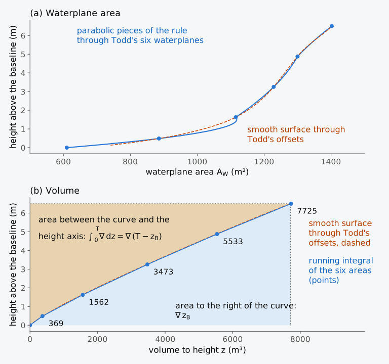
Figure 2.12 The Series 60 hull from Todd’s table and from the smooth surface (dashed): (a) waterplane area against height; (b) volume to each height, with the two areas that give the centre of buoyancy shaded.
2.8.2 The centre of buoyancy from the volume curve
The volume curve also gives the height of the centre of buoyancy. The vertical moment of the volume below a waterline at height is , and since is the volume of the layer between and , integration by parts turns it into an integral of the volume curve:
where is the volume up to height and its value at . In Fig. 2.12(b) the integral is the area between the volume curve and the height axis. The curve divides the rectangle of height and width into that area, , and the area to its right, , so the depth of the centre of buoyancy below the waterline is the first area divided by the volume4,8. Once the volume curve has been computed as a running integral, this relation gives with one more integration and no moments (Exercise 2.18); it needs the curve to be well defined at its lower end, where it is least reliable.
2.9 Other rules and methods
Everything so far has taken the ordinates where the table of offsets gives them, at fixed stations and waterlines. The rules below either use more of those ordinates at once, or place the ordinates where a surface that can be cut anywhere allows, or do without ordinates, by describing the section as a polygon or tracing it with an instrument. The rules used so far belong to a family, the Newton–Cotes rules, which integrate the polynomial through equally spaced ordinates. With five ordinates the family gives Boole’s rule, exact for polynomials of degree 5, with weights proportional to 7, 32, 12, 32 and 7; Hamlin8 tabulates the family up to nine ordinates. Adding ordinates does not improve the family indefinitely. The nine-ordinate rule, and every rule with eleven or more, has negative weights. The absolute values of its weights then add up to more than the length of the base, and errors in the ordinates can be amplified rather than averaged. For tables of offsets, composite Simpson rules on closely spaced stations are the better choice.
2.9.1 Tchebycheff and Gauss rules
Two other families drop the equal spacing. The Chebyshev rules, which naval architecture traditionally spells Tchebycheff, give all the ordinates equal weights and place them where equal weighting is most accurate. A hand calculation with them needs no multipliers, only a sum, and this was their attraction when ordinates were measured from a drawing8,9. For two ordinates, measure from the middle of a base of half-length , and place the ordinates at , each with the weight . Odd powers of are then integrated exactly by symmetry, and the rule must also integrate 1 and exactly:
so that and . The area is the mean of the two ordinates times the length of the base, and since is integrated exactly as well, two ordinates are exact for cubics, as the three of Simpson’s first rule are. With more ordinates the conditions become equations of higher degree in the positions, whose solutions are tabulated (Table 2.5). Classical Tchebycheff rules, in which equally weighted ordinates integrate every polynomial up to degree exactly, have all their ordinates real for up to seven ordinates and for nine, and for no other number15. The eight- and ten-ordinate Tchebycheff spacings in the tables of Hamlin and Tupper are two four- or five-ordinate rules placed side by side on the two halves of the base. The Gauss rules choose both the positions and the weights, and ordinates then integrate a polynomial of degree exactly, the highest degree that ordinates can reach; the positions are the roots of the degree- Legendre polynomial9,15. For two ordinates the Gauss and Tchebycheff rules coincide, and three Gauss ordinates are as exact as the five of Boole’s rule.
Table 2.5 Positions of the ordinates of the Tchebycheff and Gauss rules, as fractions of the half-length of the base measured from its middle, and the weights of the Gauss rules as fractions of the length of the base. Each Tchebycheff ordinate has the weight ; the integral is the length of the base times the weighted sum of the ordinates.
| Ordinates | Tchebycheff positions | Gauss positions | Gauss weights |
|---|---|---|---|
| 2 | ±0.57735 | ±0.57735 | 0.50000 |
| 3 | 0; ±0.70711 | 0; ±0.77460 | 0.44444; 0.27778 |
| 4 | ±0.18759; ±0.79465 | ±0.33998; ±0.86114 | 0.32607; 0.17393 |
| 5 | 0; ±0.37454; ±0.83250 | 0; ±0.53847; ±0.90618 | 0.28444; 0.23931; 0.11846 |
Positions that are not equally spaced are of no use for a table of offsets measured at fixed stations, but they are useful when the hull is a surface that can be cut anywhere, as it is in every modern design system. The rules, each with five ordinates or fewer, are compared on two integrands in Table 2.6. On Chapman’s smooth arc the errors fall as the degree of exactness rises, and the Gauss rule with five ordinates is better than Simpson’s rule by a factor of twenty thousand. On the cube of the Wigley half-breadth that ranking breaks down. Of the five-ordinate rules, only the Gauss rule is better than the trapezoidal rule, which gains here for the reason found earlier for , and Boole’s rule is the worst. Four Gauss ordinates give the exact answer, since the integrand has degree 6 and four Gauss ordinates are exact up to degree 7. The degree of exactness is a reliable guide on the arc, but not on an integrand whose slope vanishes at both ends, as that of the cubed Wigley half-breadth does; there only a test on that integrand shows which rule is better (Exercise 2.19).
Table 2.6 Errors of five rules on two integrands: Chapman’s arc, , and the cube of the Wigley half-breadth, .
| Rule | Ordinates | Exact for degree | Rule minus exact, arc (absolute) | Rule minus exact, Wigley cube (%) |
|---|---|---|---|---|
| Trapezoidal | 5 | 1 | −0.048 | +0.83 % |
| Simpson’s first | 5 | 3 | −0.00025 | −2.02 % |
| Boole | 5 | 5 | −0.000034 | −5.21 % |
| Tchebycheff | 5 | 5 | +0.000012 | +1.88 % |
| Gauss | 3 | 5 | +0.000032 | +5.00 % |
| Gauss | 5 | 9 | +0.00000001 | 0 (exact from 4 ordinates) |
Example 2.9. Tchebycheff and Gauss by hand. Find the area under Chapman’s arc, from to 4, with the two-ordinate Tchebycheff rule and with the three-ordinate Gauss rule, and compare their errors with those of the trapezoidal rule and Simpson’s rule with five ordinates, −0.048 and −0.00025.
2.9.2 Polar integration
A boundary that is closer to a circle about some point than to a curve over a straight base is integrated more accurately in polar coordinates. Take a pole O and measure the radius to the boundary at angles , in radians, measured downwards from the horizontal through O. The thin triangle between and has the area , and its centroid lies two-thirds of the way out, at across from O and below it. Adding the triangles,
where is the distance of the centroid across from O and its depth below O4,8. Any rule of this chapter evaluates the integrals, with the angular spacing as the interval and , and as the ordinates. For a transverse section the pole is usually placed on the centreline, and a radius is passed through every point where the outline turns sharply, such as the deck edge9.
The method also meets the difficulty found at the bilge of the Series 60 midship section. With the pole at the centre of the bilge radius, a circular bilge has a constant radius, which any rule integrates exactly. Seen from that centre (Fig. 2.13(b)), two of Todd’s three lowest midship offsets lie within 6 mm of the circle of Todd’s radius, and the third, at 0.075, lies 0.10 m inside it; this is the uncertainty of the table at the bilge. Radial ordinates were also used for ships heeled to large angles: Barnes’s method, introduced in 1861, found the volumes of the wedges between the upright and the inclined waterplanes by integrating over radial planes at intervals of angle4.
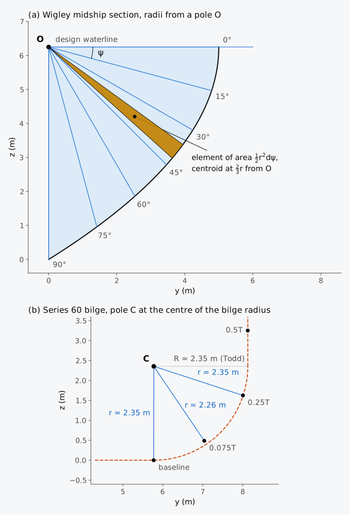
Figure 2.13 Polar integration: (a) the Wigley midship section, one side, with radii 15° apart from a pole O on the waterline; (b) the Series 60 bilge seen from the centre C of the bilge radius.
Example 2.10. The Wigley midship section in polar coordinates. From a pole on the centreline at the design waterline, the radii to the midship section of the Wigley hull ( = 10 m, = 6.25 m) at 15° intervals, from the waterline () down to the keel ( = 90°), are 5.000, 4.958, 4.890, 4.899, 5.068, 5.477 and 6.250 m (Fig. 2.13(a)). Find the area of the half-section, the depth of its centroid below the waterline and its distance from the centreline by polar integration, and compare them with the exact values , and .
2.9.3 Polygons and Green’s theorem
A section, or any other plane figure, can be described by a polygon instead of by ordinates, and the area and moments of the polygon are then found exactly. Take a closed polygon with vertices , , in order round the boundary, with vertex taken as vertex 1, and write . The triangle with its corners at the origin and at vertices and has the area , positive when its corners run counter-clockwise and negative otherwise, and its centroid is at a third of the sum of the two vertices. Added over all the edges, the triangles cover the polygon once; where they reach outside it, triangles of opposite signs cancel. The area and its first moments are therefore
which is Green’s theorem, turning an integral over an area into an integral round its boundary, applied to straight edges14. The triangles also give the second moments. A point of the triangle can be written with and , an element then has the area , and the integrals of , and over that unit triangle are 1/12, 1/24 and 1/12. For one triangle, therefore,
and, over all the edges,
These are second moments about axes through the origin, which the parallel-axis theorem moves to the centroid. Written in for a waterplane instead of for a section, these sums give the second moments of a waterplane of any shape, including the product of inertia when the waterplane is not symmetric about the centreline, which Chapters 8 and 12 need (Exercise 2.20).
The vertices are taken counter-clockwise when is drawn to the right and upwards. Since points to port, this is the section seen from forward. Taken the other way round, each of these sums changes sign; the area comes out negative, but the centroid, a ratio of two sums, is unchanged. Applied to the half-section through Todd’s six midship ordinates, closed along the centreline and the waterline, Green’s theorem gives 51.22 m², as the trapezoidal rule does, since both join the six ordinates by straight lines. The polygon is useful because it can have any shape and can be cut by a waterline at any angle; the heeled sections of Chapter 8, whose immersed parts are bounded by the hull on one side and an inclined waterline on the other, are integrated in this way (Fig. 2.14). As the vertices are brought closer together, the polygon converges to the curve at the rate of the trapezoidal rule.
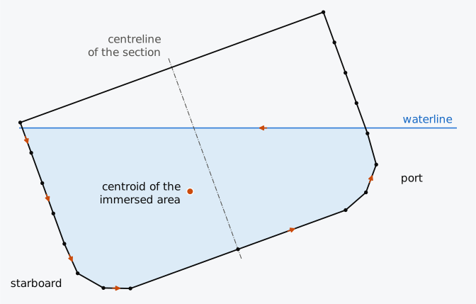
Figure 2.14 The Series 60 midship section as a polygon, seen from forward and heeled 20° to starboard. The arrows show the counter-clockwise order of the vertices of the immersed part.
2.9.4 The planimeter
Before computers, areas were also measured mechanically. The polar planimeter, the form most used in naval architecture, was invented by Jakob Amsler-Laffon in the 1850s8,14. It has two arms hinged together (Fig. 2.15). The pole arm turns about a point held down by a weight. The tracer arm carries a measuring wheel whose axis lies along the arm, and the wheel therefore rolls only with the part of the motion that is across the arm. When the tracer point is taken once round an outline, with the pole outside it, the distance rolled by the wheel is the enclosed area divided by the length of the tracer arm. The wheel adds up a line integral round the boundary, and the instrument works because of Green’s theorem, which turns such an integral into the area inside, as it does for a polygon14. On a body plan, the tracer was taken round each section up to the waterline in turn, or, to save work, round the two end sections together, then round all the sections with Simpson’s multiplier 4 and then all those with 2; the three readings, multiplied by 1, 4 and 2, gave the volume4. Amsler’s integrator, a development of the planimeter, gave the first and second moments of the area as well7, and its main use was for the cross curves of stability8, the subject of Chapter 8.
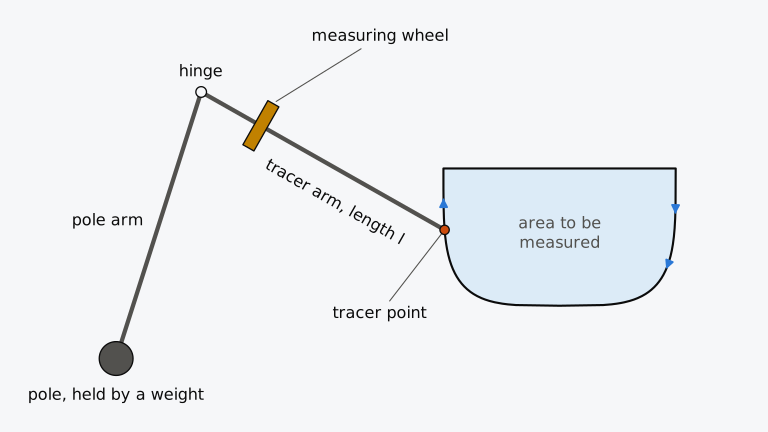
Figure 2.15 The polar planimeter (schematic). The tracer point is taken clockwise round the outline, with the pole outside it; the area is times the distance rolled by the wheel.
Historical note: the planimeter
The sources differ on the year in which the Swiss Jakob Amsler-Laffon (1823–1912) invented the polar planimeter. Biran14 gives 1854, and Biran and López-Pulido7 1856. Hamlin8 writes about 1856. Amsler gave a proof that the instrument measures the area, and other proofs followed in the next decades, but Guido Ascoli, in a report of 1947, was the first to relate it to Green’s theorem14. Amsler went on to develop the integrator. The first properly working one reached Britain in 1878, and it shortened stability calculations considerably while being simple enough to be operated by apprentices14.
2.9.5 Integration by computer
Hydrostatics programs did not at once abandon the table of offsets. The US Navy’s Ship Hull Characteristics Program, described in 1988 as widely used in American design offices and shipyards, took offsets at 2 to 29 points on each station and integrated each section by Simpson’s first rule8. Programs today usually work from a surface model of the hull instead17. One approach fits a spline through the offsets, or takes the spline surface of the design system, and integrates it, either exactly or by a rule on a much finer grid than any table; the smooth surface, built from shape-preserving cubics, was integrated in the second way. Another approach describes each section as a polygon and integrates the polygon exactly, by Green’s theorem.
Simpson’s rule on the offsets does not give the integral of a spline through them, although the rule is exact for a cubic. An interpolating spline usually changes from one cubic to the next at every data point17. Each Simpson pair spans two cubics, whose cubic terms on the two sides of the middle ordinate no longer cancel. On the Series 60 design waterline the rule gives 1402.12 m² between the perpendiculars and the smooth surface 1401.92 m². The difference is small because the waterline is smooth and the stations are close; the rule does not integrate the spline exactly.
The volume of a closed surface can be found from its triangles by the divergence theorem, the three-dimensional counterpart of Green’s theorem, as was done in Chapter 1 to check the Series 60 surface. Whatever the method, a hydrostatics program should be tested first on a hull with exact answers and then by refining its spacing until the results stop changing. A comparison with an independent calculation, such as Todd’s displacement, completes the test. Simpson’s rule applied by hand to a few sections and waterplanes cut from the program’s own model of the hull is such a calculation, independent of the program’s integration, although not of its model.
2.10 Hydrostatic integration in industry today
Most of the rules of this chapter were made for hand calculation from a table of offsets. What has passed into software is mostly the approaches of Sec. 2.9, applied to a surface model or a mesh, and the testing against known answers. Simpson’s rule itself, once worked by hand, is also implemented in programs14. A rule such as those of this chapter is still needed wherever a quantity is known only at fixed points, as when a stability instrument stores its stability data at fixed angles of heel and reports the areas under the curve of righting levers16. The table of offsets is also still accepted for approval. When a stability instrument is approved for a particular ship, the International Code on Intact Stability, 2008 (the IS Code; Resolution MSC.267(85)) allows the hull form to be submitted as a table of offsets, among other forms, where the program needs it to model the ship18. The practice described here is that of 2026, and the section is revised with each release. Programs are named only as documented examples of methods that many systems share.
2.10.1 Sections, polygons and meshes
Few makers of hydrostatics programs state the rules they use, but several document whether their programs integrate polygonal sections or a mesh. The GHS program represents each volume by a series of closed polylines at stations19, that is, by polygonal sections such as those integrated by Green’s theorem. Orca3D computes its hydrostatics on a mesh of the surface model. Since version 2.0.18 of 2020 the user has been able to display and adjust that mesh20. In the research solver Calcoque the displacement and its centre are computed by cutting a watertight volume mesh with the waterplane21. Two open-source libraries show their methods in their source code. Capytaine computes the volume of a mesh as a sum over its faces, by the divergence theorem22,23. Meshmagick takes the waterplane area and its moments from the polygon in which the waterplane cuts the mesh, by boundary sums like those of Green’s theorem for a polygon24.
2.10.2 Stability instruments
The integrals are also evaluated on board, by a stability instrument. MSC.1/Circ.1229 defines a stability instrument as the hardware and software fitted to one particular ship to show, for whatever loading condition the ship is in, whether it meets the stability requirements of its own stability booklet16. The loading condition is the cargo, ballast, fuel and stores on board at the time, and where they are stowed. The instrument’s software is approved for that ship once the accuracy of its results, and of the ship data it uses, has been verified16. Oil and chemical tankers, among others, must carry such an instrument under MARPOL Annex I and the IBC Code, unless the Administration, the government of the state whose flag the ship flies, waives the requirement25. The requirement applies to such tankers constructed on or after 1 January 2016, and to existing tankers from their first scheduled renewal survey on or after that date (the periodic survey at which a ship’s certificates are renewed), but not later than 1 January 2021, as set out in Resolution MEPC.248(66) and MGN 611 (M)25,26. According to MGN 611 (M), a waiver may be granted, for example, to a tanker on a dedicated service with a few approved loading conditions, or to a tanker whose stability is checked remotely by a method the Administration has approved; such a ship shows compliance by that method instead25.
Classification societies set technical rules for the construction and maintenance of ships and check by survey that the ships registered with them meet those rules. The International Association of Classification Societies (IACS) sets a unified requirement for onboard stability software, IACS UR L5, Rev. 4, issued in 2020. UR L5 does not itself require a stability instrument to be fitted; it specifies the requirements for the software where one is fitted27. UR L5 distinguishes four types of software, from Type 1, which calculates intact stability only, the stability of the undamaged ship, to Type 4. Type 4 calculates damage stability, the stability of the ship with one or more compartments flooded (Chapter 12), for the actual loading condition and an actual flooding case, the set of compartments actually flooded, to give operational information for a safe return to port of the damaged ship. For Types 3 and 4 the damage stability must be calculated directly from a full three-dimensional model of the hull (UR L5, Section 3). For approval on a particular ship, the society and the applicant agree at least four loading conditions from the approved stability information, the hydrostatic and stability data approved for the ship and supplied to its master. The results for these conditions must agree with that information within set tolerances, and for Type 4 software for a safe return to port the society also checks at least three damage cases, each with at least three loading conditions (UR L5, para. 6.2).
The tolerances of MSC.1/Circ.1229 depend on how the program obtains its results. A program that uses only data stored from the approved stability information should print those data exactly. Its results may differ from the approved ones only by rounding or abridged input, or, after review by the Administration, where it uses data for trims other than those of the approved information16. A program that computes from a model of the hull is compared with the approved stability information or with the model used by the approving authority, and its results must agree within the tolerances that the Circular tabulates, each percentage being taken of the approved value16. Table 2.7 gives them, as the Circular prints them in the table that follows its para. 4.6, for the quantities used in the following chapters16: the displacement may differ by up to 2 %, the vertical centre of buoyancy by 1 % / 5 cm max and the areas under the curve of righting levers by 5 % or 0.0012 m·rad. The Circular does not say how the two values of such a tolerance are combined. IACS UR L5 prints the same pairs of values, without “max”, and states that where a tolerance has two values the allowable tolerance is the greater of the two27. Larger differences are accepted only where the Administration finds them satisfactorily explained and without adverse effect on the safety of the ship16.
Table 2.7 Tolerances of MSC.1/Circ.1229 for a stability program that computes from a model of the hull, for the quantities of the following chapters, in the Circular’s form; a percentage is of the approved value16. Where a tolerance has two values, IACS UR L5 allows the greater of the two27.
| Quantity (chapter where treated) | Tolerance |
|---|---|
| Displacement (Chapters 2 and 3) | 2 % |
| Draughts, forward, aft and mean (Chapter 3) | 1 % / 5 cm max |
| Longitudinal centres of buoyancy and flotation, from the AP (Chapter 2) | 1 % / 50 cm max |
| Vertical centre of buoyancy (Chapter 2) | 1 % / 5 cm max |
| Height of the transverse metacentre above the keel, KM, the Circular’s “transverse metacentric height” among its hull-form data (Chapter 4) | 1 % / 5 cm max |
| Moment to change trim 1 cm (Chapter 6) | 2 % |
| Cross curves of stability, KN (Chapter 8) | 50 mm |
| Free surface correction (Chapter 5) | 2 % |
| Metacentric height, GM (Chapter 4) | 1 % / 5 cm max |
| Righting levers, GZ (Chapter 8) | 5 % / 5 cm max |
| Areas under the curve of righting levers (Chapters 9 and 11) | 5 % or 0.0012 m·rad |
Recent programs compute from three-dimensional models of the hull and its compartments. In July 2022 the classification society DNV type-approved NAPA Stability, onboard software for passenger ships. Type approval certifies that the design of a product meets stated requirements, here DNV’s own intact and damage stability requirements, the UR L5 Type 4 requirements for a safe return to port and those of DNV’s class notation LCS(DC), an optional addition to a ship’s classification that records that it meets further rules28. Bureau Veritas offers software of all four types with calculations “based on 3D ship models”29. Liu et al.30 describe a direct damage stability method for a Type 3 onboard loading computer, that is, a stability instrument, in which the hull and the compartments are stored as STL triangle meshes. For an asphalt tanker of 7500 t deadweight, the mass of cargo, fuel and stores it can carry, they calculated 18 loading conditions, each with one damage case, and compared the results with the ship’s loading manual, a document that the ship carries on board and that a loading computer supplements7. The mean difference in GZ was 0.002 m and the largest 0.013 m. These figures describe that test only and do not establish the accuracy of such software in general.
2.10.3 Testing hydrostatics software
A published study illustrates testing by comparison with independent calculations. Dawson31 compared the tank tables, the volume and centre of a tank’s contents at each depth of filling, that Maxsurf Stability computes for four identical cubic tanks in a box-shaped benchmark barge with those of two other programs, Paramarine and Rhinoceros 3D. Such shapes also have exact answers, against which the programs can be tested as well.
2.11 From geometry to hydrostatics
You can now evaluate every integral of Table 2.1 from a table of offsets, a surface or a polygon, and say how far to trust the result. In Fig. 2.16 those integrals are grouped by the waterplanes, sections or volumes over which they are taken, with the later chapters that use them. In Chapter 3 the displacement volume and the volume curve are set against the weight of the ship, to find the draught at which it floats, and the centre of buoyancy against the centre of gravity. Chapman began from the comparison of displacement and weight, in which the weight of the cargo is the difference between the displacement and the weight of the hull and rigging. In Chapter 4 the transverse second moment of the waterplane gives the metacentric radius, and the longitudinal second moment gives the longitudinal metacentric radius, from which Chapter 6 finds the trim. Chapter 5 applies these integrals to the liquid in tanks and Chapter 12 to flooded compartments. Chapter 7 repeats them at every draught and Chapter 8 at every angle of heel. Chapter 9 integrates the righting lever over the angle of heel, and Chapter 11 sets minimum values for the area under its curve. Each of these steps uses the rules of this chapter and the checks of Sec. 2.7, whether the hull is described by offsets, a surface or a polygon.
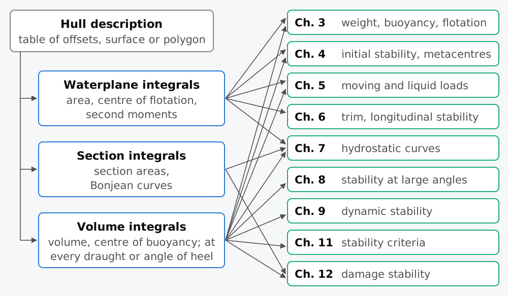
Figure 2.16 Where the integrals of Chapter 2 lead. Each arrow from the hull description is an integral evaluated by a rule of this chapter.
Summary
The quantities of hydrostatics are integrals of half-breadths. A hull is known only at a finite number of points, and each of these integrals is evaluated by a rule that is a weighted sum of ordinates. The trapezoidal rule joins the points by straight lines and is of order 2 on a smooth curve. Simpson’s first rule, with which Chapman began his treatise, fits parabolas to pairs of equal intervals, is exact for cubics and is of order 4 on such a curve. Half stations, the second rule, the rule for unequal intervals and the five-eight rule extend it to the spacings that real tables have, and a part beyond the last ordinate is added with an extra ordinate or an assumed shape, on which the result depends.
These rules also give first and second moments, from the moments of a strip, with care for integrands such as , and the parallel-axis theorem moves a second moment to the centroid; the inertia coefficients compare the second moments of a waterplane with those of its rectangle . A volume is integrated twice, on a displacement sheet whose two grand totals agree by construction, and their agreement checks only the arithmetic; the centre of buoyancy follows from moments of the sections or of the waterplanes, or from the area between the volume curve and the height axis.
Tchebycheff and Gauss rules choose the positions of the ordinates and need fewer of them, and polar coordinates suit an outline that is nearly a circle about a point, such as a bilge. Green’s theorem gives the area and moments of a polygon of any shape, with its vertices taken in counter-clockwise order, and the planimeter also rests on it.
Accuracy is judged by test cases with exact answers and by repeating the calculation at a different spacing or with a different rule; where the curve has a corner or a vertical tangent, the order falls and the estimate must be checked. These results give seven rules for practice:
- choose the rule from the spacing: Simpson’s first rule for equally spaced ordinates and an even number of intervals (an odd number of ordinates), the second rule for three equal intervals, and the rule for unequal intervals, preferably with neither interval of a pair more than twice the other, since otherwise one of its weights is negative and errors in the ordinates can be amplified; where the table fixes such a pair, as Todd’s waterlines at 0, 0.075 and 0.25 times the draught do, the rule can still be used, with the negative weight noted; where the ordinates can be placed anywhere, as on a surface, a Gauss rule needs the fewest, once a test on the integrand has confirmed it;
- test any integration scheme on a hull whose integrals are known exactly before trusting it;
- plot every curve of areas and look for a point off a fair curve, or, where the values are equally spaced, for a second difference out of line, since an error in the offsets passes every check of the arithmetic;
- put an ordinate at every knuckle, chine or end of a flat, and closer ordinates where the curve turns sharply;
- treat the parts of the hull beyond the end ordinates separately, and state the shape assumed for them;
- when moving a second moment to the centroid, subtract the area times the square of the distance;
- estimate the error by repeating the calculation with a different spacing, and check the order before extrapolating.
Notes on the data
Chapman’s treatise. The quotations are our translations of the French edition1; its numbers are given as printed.
Wigley hull. The offsets, radii and other data of the Wigley hull in this chapter are computed from its formula, Eq. (1.5).
Series 60. Values are computed from the offsets of Todd6, up to the design waterline. Values of the smooth surface are given for comparison only, as is its ending of the design waterline aft of the AP in Fig. 2.6, which is a choice made in Chapter 1 and not part of Todd’s data. Stations are numbered from the AP, the reverse of Todd’s numbering. The displacement sheet of the Series 60 hull, in the layout of Table 2.4 with the weights for Todd’s waterlines up the height, is in the chapter’s data file series60_displacement_sheet.csv; it reproduces = 7719.9 m³ and = 3.48 m. The section areas of Exercise 2.16 are computed from Todd’s offsets with the rule of Example 2.8 and rounded to 0.1 m²; Exercise 2.21 alters one of them on purpose.
Exercises
Under each exercise, “Show answers” opens its short answers and “Show full solution” its worked solution; an exercise without answer boxes gives its short answers in brackets at its end. Exercises 2.1 to 2.7 are adapted from Attwood4 (public domain). Use = 1025 kg/m³ for sea water.
2.1 A curve has ordinates 0.4 m apart of 3.31, 4.12, 4.44, 4.59, 4.65, 4.66 and 4.64 m. Find the area under it by Simpson’s first rule and by Simpson’s second rule. Adapted from Attwood4.
2.2 A curve has ordinates 5.5 m apart of 1.89, 4.21, 6.68, 8.05, 6.81, 4.48 and 2.24 m. Taking the result of Simpson’s first rule as correct, find the percentage error of the trapezoidal rule and of Simpson’s second rule. Adapted from Attwood4.
2.3 A quadrant of a circle of radius 1 m is divided by ordinates parallel to one radius, at distances 0.25, 0.5, 0.625, 0.75, 0.8125, 0.875 and 0.9375 m from it, as well as the radius itself and the point where the arc meets the other radius. Find the area (a) exactly, (b) with the ordinates 0.25 m apart only, (c) adding the ordinates at 0.625 and 0.875 m, (d) with all the ordinates, and (e) with all except the ordinate at 0.625 m, using the second rule from 0 to 0.75 m. Comment on the results. Adapted from Attwood4.
2.4 The waterplane areas of a vessel, 0.45 m apart from the load waterline downwards, are 186, 186, 149, 116 and 28 m². Neglecting the small volume below the lowest, find the displacement volume and the displacement mass in sea water. Adapted from Attwood4.
2.5 The half-breadths of a waterplane, 4.6 m apart from the after end, are 1.58, 3.11, 4.39, 5.46, 6.28, 6.92, 7.41, 7.77, 7.99, 8.08, 8.11, 8.02, 7.74, 7.28, 6.64, 5.73, 4.69, 3.51, 2.19, 1.01 and 0.67 m. Find the area of the waterplane and the position of its centre of flotation relative to the middle ordinate. Adapted from Attwood4 (one ordinate corrected).
2.6 A plane area bounded by a curve and a straight base has ordinates 1.2 m apart of 0, 3.81, 4.36, 4.60, 4.72, 4.69, 4.51, 4.27 and 0 m. Find its area, the distance of its centroid from the first ordinate, and its height above the base. Adapted from Attwood4.
2.7 The half-breadths of a waterplane, 8.5 m apart, are 0.02, 1.42, 3.06, 4.36, 5.11, 5.38, 5.30, 4.94, 4.13, 2.94 and 1.11 m. Find its transverse second moment about the centreline by Simpson’s rule and by the trapezoidal rule, and explain why the two are so close. Adapted from Attwood4.
2.8 Derive the rule for a pair of unequal intervals, Eq. (2.9), by integrating the parabola through three ordinates at 0, and , and show that it reduces to Simpson’s rule when . Then derive the five-eight rule and show that the five-eight areas of the two halves of a Simpson pair add up to the Simpson area. [; and ]
Show full solution
The conditions. A rule integrates every parabola exactly if it integrates 1, and exactly. With the ordinates at , and ,
The weights. Subtracting times the second equation from the third leaves , so
the second from the second equation and the third from the first: the weights of the rule for unequal intervals. For intervals of 1 and 3, for example, they are , and , and the first is negative because .
Equal intervals. With the weights become , which is Simpson’s rule.
The five-eight rule. Integrating the parabola through the three ordinates, with , from 0 to only gives , which is the five-eight rule; from to it gives, by symmetry, . The two add up to
2.9 Show that Simpson’s rule is exact for on , and find the constant in its error formula, Eq. (2.7), by applying the rule to on . Find the constant of the second rule from as well, and show that it is . [; ]
Show full solution
A cubic. For on the integral is zero, and the rule gives .
The constant of the first rule. For the integral is and the rule gives , so that . In the error formula, and , so
The constant of the second rule. On the integral of is and the rule gives , so the error is . With ,
2.10 For the Wigley waterline, with , show that Simpson’s rule with intervals gives the longitudinal second moment about amidships, , with a relative error of exactly , and evaluate it for . [−0.16 %]
Show full solution
The integral. With , the second moment about amidships is with , whose exact integral is .
The error. The fourth derivative of is the constant −24, so the error formula of Simpson’s rule is exact. With spacing in ,
The rule gives the integral minus , and its relative error is .
Comment. For this is −0.0016, or −0.16 %, the error quoted for of the Wigley waterplane.
2.11 For a function whose slope is zero at both ends of the interval, the term of the error of the trapezoidal rule vanishes. Using the expansion , predict the error of the trapezoidal rule with ten intervals for of the Wigley design waterplane, with , = 100 m and = 10 m, and compare it with the actual error of the rule, −0.88 m⁴. [−0.89 m⁴, against −0.88 m⁴]
Show full solution
The derivatives. The integrand is with m³, and at both ends. In , , which is at the FP () and at the AP, so ; with in m³ and in m, has no unit.
The error. With = 10 m,
the rule exceeds the integral by 0.89 m⁴.
Comment. The actual error is m⁴; the small difference is the next term of the series.
2.12 The trapezoidal rule gives 43.713, 47.931 and 49.437 for the area of Chapman’s quadrant of radius 8 with ordinates 4, 2 and 1 apart. Estimate the order of convergence from the three results, and an improved value by Richardson extrapolation. Then extrapolate the last two results with , the order of the trapezoidal rule on a smooth curve, and compare with Simpson’s rule on the nine ordinates 1 apart.
2.13 The waterplane areas of the Wigley hull, = 100 m, = 10 m and = 6.25 m, are with . At five waterlines 1.5625 m apart, from the keel to the design waterline, find the volume up to each waterline by the running Simpson integral, and compare with the exact . Explain why the results are exact even at the odd waterlines. [238.7, 868.1, 1757.8 and 2777.8 m³, all exact]
Show full solution
The waterplane areas. The areas at = 0, 1.5625, 3.125, 4.6875 and 6.25 m are 0, 291.67, 500.00, 625.00 and 666.67 m², and = 1.5625 m.
The running integral. Up to the first waterline by the five-eight rule, up to the second by Simpson’s rule, and so on:
Comment. The four values agree with the exact formula. The waterplane area of the Wigley hull is a parabola in , and both the five-eight rule and Simpson’s rule are exact for a parabola.
2.14 The half-section of a barge is a polygon with vertices at = (0, 0), (4, 0), (5, 1), (5, 3) and (0, 3) m, taken counter-clockwise. Find its area and the height of its centroid by Green’s theorem, and check both by dividing the section into two rectangles and a triangle.
2.15 At intervals of 7°, the righting levers of HMS Captain and HMS Monarch, the two ships of the prologue of Chapter 1, were as follows4:
| (°) | 0 | 7 | 14 | 21 | 28 | 35 | 42 |
|---|---|---|---|---|---|---|---|
| , Captain (m) | 0 | 0.108 | 0.216 | 0.273 | 0.254 | 0.197 | 0.133 |
| , Monarch (m) | 0 | 0.102 | 0.210 | 0.311 | 0.464 | 0.552 | 0.559 |
Find the area under each curve up to 28° and up to 42°, in metre-radians, and the area between 28° and 35° by the five-eight rule. Multiplied by the ship’s weight, such an area is the work needed to heel the ship to that angle (Chapter 9), and Chapter 11 sets minimum values for it. Compare the two ships.
2.16 At a ballast draught of 4.877 m, three-quarters of its design draught, the immersed section areas of the Series 60 hull at its even-numbered stations, 12.192 m apart from the AP (station 0) to the FP (station 20), are 0, 16.8, 41.9, 63.6, 74.5, 76.7, 72.7, 57.8, 34.7, 14.1 and 0 m². (a) Find the displacement volume and the displacement mass in sea water by Simpson’s first rule. (b) Find the position of the centre of buoyancy relative to amidships. (c) Taking the largest section as the midship section, find the prismatic coefficient at this draught. (d) Find the volume by the trapezoidal rule, and its difference from (a) as a percentage, and explain why the difference is small. (e) The volume to the ballast draught found from the waterplanes, which use all 25 stations, is 5533.2 m³. Explain the difference from (a).
2.17 The Wigley hull, = 100 m, = 10 m and design draught = 6.25 m, has the half-breadths , with and . Set out a displacement sheet, in the layout of Table 2.4, for the hull floating at half its design draught, 3.125 m, with eleven stations 10 m apart and five waterlines 0.78125 m apart from the keel. Find the volume by sections and by waterplanes, the longitudinal centre of buoyancy, and the height of the centre of buoyancy above the keel, with the check from the waterline. Compare the height with the exact value, 0.325 times the design draught.
2.18 (a) The waterplane areas of a vessel, 0.45 m apart from the load waterline downwards, are 186, 186, 149, 116 and 28 m². Find the height of the centre of buoyancy above the lowest waterplane from the moments of the waterplane areas, and check it by moments about the load waterline. (b) Find the volume up to each waterplane by the running Simpson integral, and from these volumes the depth of the centre of buoyancy below the load waterline, from the area between the volume curve and the height axis. (c) The volumes of the Wigley hull up to its waterlines at 0, 1.5625, 3.125, 4.6875 and 6.25 m above the keel are 0, 238.7, 868.1, 1757.8 and 2777.8 m³. Find from them by Eq. (2.18), and compare it with .
2.19 Tupper9 states that the four-ordinate Tchebycheff rule is more accurate than the five-ordinate Simpson rule. Test the statement on Chapman’s arc, , and on the cube of the Wigley half-breadth, , and explain the result. The four ordinates of the Tchebycheff rule stand at ±0.18759 and ±0.79465 of the half-length of the base from its middle.
2.20 The half-section of a barge is a polygon with vertices at = (0, 0), (4, 0), (5, 1), (5, 3) and (0, 3) m, taken counter-clockwise. Find , and by Green’s theorem, and check the first two by dividing the section into two rectangles and a triangle. Then find the second moment of the half-section about a horizontal axis through its centroid.
2.21 At a ballast draught of 4.877 m, the immersed section areas of the Series 60 hull at its even-numbered stations, 12.192 m apart from the AP (station 0) to the FP (station 20), were entered on a sheet as 0, 16.8, 41.9, 63.6, 74.5, 76.7, 77.2, 57.8, 34.7, 14.1 and 0 m², with two digits of one value interchanged. (a) Find the second differences of the areas and locate the faulty value. (b) The correct value is 72.7 m². Find, by Simpson’s first rule, how much the faulty value changes the displacement volume and the position of the centre of buoyancy. (c) Had the area of that station come out too large from a mistyped offset on a displacement sheet, the two grand totals of the sheet would still agree. Explain why.
2.22 The Wigley hull, = 100 m, = 10 m and = 6.25 m, has a tank on the port side of a centreline bulkhead, between stations 3 and 7, 30 m and 70 m from the AP, whose outer boundary is the hull side. The liquid in it stands at the height of the design waterline, where the half-breadths at stations 3, 4, 5, 6 and 7, 10 m apart, are 4.2, 4.8, 5.0, 4.8 and 4.2 m. For the free surface of the liquid, find by Simpson’s rule (a) its area, (b) the distance of its centroid from the centreline, (c) its second moment about the centreline, and (d) its second moment about the longitudinal axis through its centroid.
Symbols introduced in this chapter
| Symbol | Meaning | Unit |
|---|---|---|
| area of a plane figure, a polygon or a polar figure | m² | |
| , twice the signed area of the triangle of edge and the origin | m² | |
| , | transverse and longitudinal inertia coefficients, and | – |
| distance between two parallel axes | m | |
| depth of the centroid of a figure below the pole, in polar integration | m | |
| , | error of the trapezoidal rule and of Simpson’s rule: integral minus rule | as the integral |
| ; , , , | integrand, a function of ; its first to fourth derivatives, each dividing the unit of by one more power of the unit of (for a half-breadth in m against in m: m, –, m⁻¹, m⁻², m⁻³; for : m³, m², m, –, m⁻¹) | unit of ; unit of over m, m², m³, m⁴ |
| ; | spacing of the ordinates (station or waterline spacing); waterline spacing on a displacement sheet | m |
| , | lengths of two neighbouring, possibly unequal, intervals | m |
| transverse second moment of the waterplane area, about the centreline | m⁴ | |
| longitudinal second moment of the waterplane area, about the transverse axis through F | m⁴ | |
| , | second moment of the waterplane area about a transverse axis amidships; about the transverse axis through the AP | m⁴ |
| ; | index of an ordinate; index of a waterline or of a vertex of a polygon | – |
| station number, used as a lever in units of | – | |
| length of the tracer arm of a planimeter | m | |
| first moment of a plane area about an axis | m³ | |
| ; , | multiplier (weight written as a small number with a common factor outside); weight in and in | –; m |
| number of vertices of a polygon | – | |
| number of intervals; number of ordinates of a Tchebycheff or Gauss rule | – | |
| order of a rule: its error falls as | – | |
| , , , , | value given by a rule; by the trapezoidal rule and Simpson’s rule; with spacing and | as the integral |
| bilge radius | m | |
| , | radius from a pole and its angle below the horizontal through the pole | m, rad |
| half-length of the base of a Tchebycheff or Gauss rule | m | |
| , | coordinates in a triangle of a polygon | – |
| an unknown point within the interval of integration, in the error formulae | m | |
| ordinate: half-breadth, area or other integrand at | m, m², … | |
| running integral: the approximation to | as the integral | |
| , , | coordinates of the centroid of a plane area | m |
| , | weights of the outer and inner ordinates of the second rule | m |
| variable of integration: a distance from the centreline or a height | m | |
| , | position, from the middle of the base, and weight of a two-ordinate Tchebycheff rule | m |
| displacement volume up to the height | m³ |
Corrections
Corrections to version 1.0, released on 3 November 2026, with their dates.
- 5 November 2026. The prologue gives the spacing of the seven waterlines of Chapman’s privateer as 1.62 feet, as his displacement sheet prints it, in place of 1.02 feet.
- 5 November 2026. The route for a first reading includes Sec. 2.4, whose rules Secs. 2.5 to 2.8 use.
- 5 November 2026. Sec. 2.9.2 cites Attwood for the radial planes of Barnes’s method, in place of a reference to Chapter 8, which does not describe them. Sec. 2.4.4 gives Attwood’s five-eight areas also before rounding, and the alt text of Fig. 2.10 marks the heights as fractions of the draught.
- 5 November 2026. Sec. 2.10.2 and Table 2.7 give the tolerances of MSC.1/Circ.1229 as the Circular prints them, such as 1 % / 5 cm max, in place of “1 % or 5 cm”, and give the greater of the two values as the reading of IACS UR L5; the Circular does not say how the two values combine.
References
- Chapman, F. H. af. (1781). Traité de la construction des vaisseaux (H.-S. Vial du Clairbois, Trans.). Malassis. (Original work published 1775 as Tractat om Skepps-Byggeriet; public domain.) https://archive.org/details/bub_gb_KdnWSHfxqmUC Cited: ↑ translator's preface · ↑ ch. I, pp. 1–2 · ↑ translator's preface · ↑ ch. I, Section 1 · ↑ ch. I, Section 1 · ↑ ch. I, Section 4 · ↑ translator's preface · ↑
- Nowacki, H., & Ferreiro, L. D. (2003). Historical roots of the theory of hydrostatic stability of ships. In Proceedings of the 8th International Conference on the Stability of Ships and Ocean Vehicles (STAB 2003) (pp. 1–30). Escuela Técnica Superior de Ingenieros Navales. Cited: ↑ pp. 24–25 · ↑ p. 25
- O’Connor, J. J., & Robertson, E. F. (2005). Thomas Simpson. MacTutor History of Mathematics Archive, University of St Andrews. https://mathshistory.st-andrews.ac.uk/Biographies/Simpson/ Cited: ↑
- Attwood, E. L. (1899). Text-book of theoretical naval architecture. Longmans, Green, and Co. (Public domain.) Cited: ↑ p. 6 · ↑ p. 7 · ↑ p. 6 · ↑ p. 10 · ↑ pp. 13–14 · ↑ pp. 12–13 · ↑ pp. 65–71 · ↑ p. 54 · ↑ pp. 55–56 · ↑ pp. 64–71 · ↑ p. 18 · ↑ p. 7 · ↑ p. 64 · ↑ pp. 15–16 · ↑ pp. 171–172 and 177 · ↑ pp. 77–79 · ↑ · ↑ ch. I, Ex. 14 · ↑ ch. I, Ex. 26 · ↑ ch. I, Ex. 48 · ↑ ch. I, Ex. 29 · ↑ ch. II, Ex. 5 · ↑ ch. II, Ex. 3 · ↑ ch. III, p. 102 · ↑ pp. 160–162
- IMO. (1974). International Convention for the Safety of Life at Sea, 1974 (as adopted, 1 November 1974). International Maritime Organization. Cited: ↑ regs. III/6(a) and III/7
- Todd, F. H. (1963). Series 60: Methodical experiments with models of single-screw merchant ships (Report No. 1712). David Taylor Model Basin. https://apps.dtic.mil/sti/pdfs/AD0419990.pdf Cited: ↑ Table 3 · ↑ Fig. 11 · ↑ Fig. 11 · ↑ · ↑ Table 3
- Biran, A., & López-Pulido, R. (2014). Ship hydrostatics and stability (2nd ed.). Butterworth-Heinemann. Cited: ↑ Section 3.2.1, p. 81 · ↑ Section 3.3.1 · ↑ Section 3.6 · ↑ Section 3.2.1, p. 82 · ↑ Section 3.4 · ↑ Section 4.2 · ↑ Section 13.1, pp. 321–322 · ↑ Section 13.1, p. 321 · ↑ Section 13.7, p. 355
- Hamlin, N. A. (1988). Ship geometry. In E. V. Lewis (Ed.), Principles of naval architecture: Vol. I. Stability and strength (2nd rev., ch. I). Society of Naval Architects and Marine Engineers. Cited: ↑ Section 4.8, p. 26 · ↑ Section 4.4, p. 24 · ↑ Section 5.7, Table 7, p. 35 · ↑ Section 4.5, p. 25 · ↑ Section 4.11, p. 28 · ↑ Section 5.7, Table 7, p. 35 · ↑ Section 5.16, p. 43 · ↑ Section 4.10, pp. 27–28 · ↑ Section 4.2, p. 23 · ↑ Section 4.2, p. 23 · ↑ Section 4.4, p. 25 · ↑ Section 5.2, p. 32 · ↑ Section 5.2, p. 32 · ↑ Section 5.3, p. 34 · ↑ Section 6.1, p. 45 · ↑ Section 5.8, pp. 36–37 · ↑ Section 5.7, p. 36 · ↑ Section 5.9, pp. 37–38 · ↑ Section 4.7, Table 3, p. 26 · ↑ Section 4.9, pp. 26–27 · ↑ Section 4.12, pp. 28–30 · ↑ Section 4.14, p. 30 · ↑ Section 4.15, p. 31 · ↑ Section 4.14, p. 30 · ↑ Section 5.16, pp. 42–43
- Tupper, E. C. (2013). Introduction to naval architecture (5th ed.). Butterworth-Heinemann. Cited: ↑ ch. 3, p. 39 · ↑ ch. 3, pp. 37–38 · ↑ ch. 4, p. 55 · ↑ app. B, p. 419 · ↑ ch. 3, pp. 41–42 · ↑ ch. 3, pp. 42–43 · ↑ ch. 3, pp. 43–44 · ↑ ch. 3, p. 43
- Virtanen, P., Gommers, R., Oliphant, T. E., Haberland, M., Reddy, T., Cournapeau, D., Burovski, E., Peterson, P., Weckesser, W., Bright, J., van der Walt, S. J., Brett, M., Wilson, J., Millman, K. J., Mayorov, N., Nelson, A. R. J., Jones, E., Kern, R., Larson, E., … SciPy 1.0 Contributors. (2020). SciPy 1.0: Fundamental algorithms for scientific computing in Python. Nature Methods, 17, 261–272. https://doi.org/10.1038/s41592-019-0686-2 Cited: ↑ · ↑
- Barrass, C. B., & Derrett, D. R. (2006). Ship stability for masters and mates (6th ed.). Butterworth-Heinemann. Cited: ↑ ch. 10
- ITTC. (2024a). ITTC dictionary of hydromechanics (Version 2024). International Towing Tank Conference. Cited: ↑ s.v. "Moment of area, second" · ↑ s.v. "Moments of inertia" · ↑ s.v. "waterplane inertia coefficients" · ↑ s.v. "waterplane inertia coefficients"
- ITTC. (2024b). ITTC symbols and terminology list (Version 2024). International Towing Tank Conference. Cited: ↑
- Biran, A. (2019). Geometry for naval architects. Butterworth-Heinemann. Cited: ↑ Section 3.5.2, p. 136 · ↑ Sections 3.5.3–3.5.7, pp. 137–146 · ↑ Section 3.8, pp. 164–165 · ↑ Section 3.8, pp. 163–169 · ↑ Section 3.10.1, p. 178 · ↑ Section 3.10.1, pp. 178–181 · ↑ Section 3.10.1, p. 178 · ↑ Section 3.10.1, pp. 178–179 · ↑ Section 3.10.1, pp. 181–182 · ↑ Section 3.9.1, p. 171
- Abramowitz, M., & Stegun, I. A. (Eds.). (1964). Handbook of mathematical functions with formulas, graphs, and mathematical tables (Applied Mathematics Series 55). National Bureau of Standards. Cited: ↑ Section 25.4 · ↑ Section 25.4 · ↑ Section 25.4
- IMO. (2007). Guidelines for the approval of stability instruments (MSC.1/Circ.1229, 11 January 2007). International Maritime Organization. Cited: ↑ annex, para. 4.6 · ↑ annex, paras. 4.2 and 4.3 · ↑ annex, Section 2 · ↑ annex, Section 3 · ↑ annex, para. 4.5 · ↑ annex, para. 4.6 · ↑ annex, para. 4.6 and table · ↑ annex, para. 4.1 · ↑ annex, para. 4.6 and table
- Letcher, J. S., Jr. (2009). The geometry of ships (J. R. Paulling, Ed.; Principles of Naval Architecture Series). Society of Naval Architects and Marine Engineers. Cited: ↑ Section 8.7, p. 37 · ↑ Section 3.5, p. 13
- IMO. (2020). International Code on Intact Stability, 2008 (2020 ed.). International Maritime Organization. (Includes the Explanatory Notes, MSC.1/Circ.1281.) Cited: ↑ Part B, para. 4.1.6.2.3.4
- Robert McNeel & Associates. (n.d.). AttachGHSData (Rhino 7 help). Retrieved October 7, 2026, from https://docs.mcneel.com/rhino/7/help/en-us/commands/attachghsdata.htm Cited: ↑
- Orca3D. (2020, October 22). New Orca3D version 2.0.19 available [Release notes, including version 2.0.18]. Retrieved October 10, 2026, from https://orca3d.com/blogs/news/new-orca3d-version-2-0-19-available Cited: ↑
- Grinnaert, F., Billard, J.-Y., & Laurens, J.-M. (2015). Calcoque: A fully 3D ship hydrostatic solver. In Proceedings of the 12th International Conference on the Stability of Ships and Ocean Vehicles (STAB 2015) (pp. 203–212). https://shipstab.org/files/Proceedings/STAB/STAB2015/Papers/5.1-3-Grinnaert.pdf Cited: ↑
- Ancellin, M. (2026). Capytaine (Version 3.0.0) [Computer software]. https://capytaine.org (Apache-2.0; source code inspected for the hydrostatic integrals.) Cited: ↑
- Ancellin, M., & Dias, F. (2019). Capytaine: A Python-based linear potential flow solver. Journal of Open Source Software, 4(36), 1341. https://doi.org/10.21105/joss.01341 Cited: ↑
- LHEEA. (2023). Meshmagick (Version 3.4) [Computer software]. École Centrale de Nantes. https://github.com/LHEEA/meshmagick (GPL-3.0; source code inspected for the waterplane integrals.) Cited: ↑
- Maritime and Coastguard Agency. (2019). Damage stability: Alternative verification method for tankers. UK interpretations and procedures (MGN 611 (M)). https://assets.publishing.service.gov.uk/media/5d303f1ae5274a14f41d28a1/MGN611.pdf Cited: ↑ Annex A · ↑ Annex A · ↑ para. 7.3 and Annex A
- IMO. (2014). Amendments to the Annex of the Protocol of 1978 relating to the International Convention for the Prevention of Pollution from Ships, 1973 (Resolution MEPC.248(66), adopted 4 April 2014). International Maritime Organization. Cited: ↑
- IACS. (2020). Computer software for onboard stability calculations (UR L5, Rev. 4, June 2020). International Association of Classification Societies. Retrieved October 9, 2026, from https://iacs.s3.af-south-1.amazonaws.com/wp-content/uploads/2022/02/17101147/ur-l5rev4.pdf Cited: ↑ · ↑ Table 1, Note 2 · ↑ Table 1, Note 2
- NAPA. (2022, July 11). DNV awards NAPA’s next-generation passenger ship stability management solution type approval. Retrieved October 10, 2026, from https://www.napa.fi/news/dnv-awards-type-approval-for-napa-stability/ Cited: ↑
- Bureau Veritas. (n.d.). Veristar Onboard. Retrieved October 7, 2026, from https://marine-offshore.bureauveritas.com/veristar-onboard Cited: ↑
- Liu, C., Huang, L., Sun, X., & Yin, Y. (2022). A direct damage stability calculation method for an onboard loading computer. Journal of Marine Science and Engineering, 10(8), 1030. https://doi.org/10.3390/jmse10081030 Cited: ↑
- Dawson, E. (2014, May). Formation Design Systems’ Maxsurf Stability tank table generator: Verification and validation study (DSTO-TR-2968, AR-015-954). Defence Science and Technology Organisation. https://apps.dtic.mil/sti/pdfs/ADA615333.pdf Cited: ↑ pp. 2–5