
Before the curves were computed by machine, KB could be found from the displacement curve itself. Attwood stated in 1899 that the area of the curve of displacement, divided by the load displacement, gives the depth of the centre of buoyancy below the load waterline, and proved it in an appendix8. The rule holds at any draught: in the notation of this chapter, the area between the curve and the draught axis up to the draught is , as an integration by parts with shows. The area was measured by a rule of integration or by planimeter and divided by the displacement, a method considered the most accurate for KB at low draughts, provided the lower end of the curve was carefully drawn5.
Figures and tables have more room in landscape.
Chapter 7: Hydrostatic curves
Version 1.0 · last revised 6 November 2026 · corrections
Prologue: the Virginia at Hampton Roads
On 8 and 9 March 1862 the Confederate ironclad Virginia fought the ships of the United States Navy in Hampton Roads1. The ironclad had been built on the hull of the steam frigate Merrimack, whose burnt upper works were removed. Over the middle of the hull a shield of pine and oak, about 2 ft (0.61 m) thick and plated with iron, was built to a length of about 180 ft (54.9 m), with its sides sloping at about 36°. For about 50 ft (15.2 m) forward and aft of the shield the deck lay under water2. The lower edge of the shield was meant to lie 2 ft under water3.
The displacement of the ship had been miscalculated, and it rode too high in the water4. Ballast of stone and pig iron was put on board to bring it down to its fighting trim1,4. Even so, on going into action the ship drew 22 ft (6.71 m) aft and 21 ft (6.40 m) forward1. The executive officer, Catesby ap R. Jones, recorded that the lower part of the shield forward was immersed only a few inches, “instead of two feet as was intended”3. By the second day of the fight the loss of the prow and an anchor, and the coal, water and stores used, had lightened the ship until the lower edge of the shield forward was awash3.
In May 1862 Norfolk was abandoned, and the officers of the Virginia tried to take it up the James River. The pilots said that the river had only 18 ft (5.49 m) of water over the bar that the ship had to cross. During the night the crew threw the coal and ballast overboard, and the unprotected deck rose out of the water2. The lower edge of the shield was now out of the water too, and, as Jones put it, “we were not in fighting condition”3. The pilots then declined to take the ship even at 18 ft, because the westerly winds of the previous days had lowered the water over the shallows1,2. The crew ran the ship ashore near Craney Island and set it on fire, and early on 11 May 1862 its magazine exploded3.
In March the Virginia floated too high to fight as designed, and in May it drew too much to be taken up the river. The draught at which a ship of known weight floats is read from its displacement curve, the first of the hydrostatic curves of this chapter. Unlike an ordinary hull, the hull of the Virginia also changed its form abruptly at one draught. Below the lower edge of the shield the waterplane was that of the whole hull, but once the deck went under, only the shield cut the water. In Sec. 7.5 we will return to the Virginia and see how such a change of form appears in the curves.
Chapters 3 to 6 mostly used hydrostatic values at one draught at a time. In this chapter we will collect them at every draught, as the hydrostatic curves, and see how they are calculated and checked. The contents of the ship’s tanks are calculated in a similar way and read on board from their soundings. We will then look at hulls whose form changes abruptly, and at simple estimates of the curves for early design. Last, we will return to the Bonjean curves of Chapter 1, which give the displacement of a ship trimmed too far for the curves of the level ship to be trusted.
In this chapter
By the end of this chapter you will be able to:
- compute and read the curves and tables, check the relations between their slopes, and judge when linear interpolation is accurate enough;
- find the volume in a tank from its sounding, and correct a sounding taken in a trimmed ship;
- find the draught and GM of a hull whose form changes abruptly;
- estimate KB, MCT 1 cm and the curves of a stretched hull for early design;
- find the displacement of a trimmed ship from the Bonjean curves.
What it assumes. You need the hydrostatic quantities of Chapters 3 to 6, and the Bonjean curves and integration rules of Chapters 1 and 2.
A first reading. Sections 7.1 to 7.5 carry the main thread. Secs. 7.2 and 7.3, on the accuracy of the curves and the checks on them, are best read closely; Example 7.1 shows linear interpolation in the tables putting KM 0.18 m too high. The early-design estimates of Sec. 7.6 and the Bonjean method of Sec. 7.7, an alternative to the level curves at large trims, can wait for a second reading, which the last two outcomes above need; the Bonjean method of Sec. 7.7.1 is used again in Chapters 12 and 13.
7.1 The hydrostatic curves of a ship
7.1.1 Quantities in the hydrostatic curves
The hydrostatic curves of a ship, also called its curves of form, give the hydrostatic properties of its hull at every draught5. They are calculated for the ship upright and at even keel, in a series of parallel waterplanes, and drawn against a vertical scale of draught with the keel at the foot of the sheet5,6. The usual set contains the displacement, as a volume and as a mass in sea water and in fresh water; the waterplane area and the tonnes per centimetre immersion; the longitudinal centres of buoyancy and flotation; the heights of the centre of buoyancy and of the transverse and longitudinal metacentres; the moment to change trim one centimetre; and the coefficients of form6. Some sets add the wetted surface and the change of displacement for one centimetre of trim by the stern5.
Each of these quantities has been met in an earlier chapter, and the displacement and KM already as curves against the draught. As functions of the draught , the volume is the running integral of the waterplane areas, , BM is and is . With in t/m³ and the lengths in metres, the TPC is in t/cm, and MCT 1 cm is taken as in t·m/cm, with in place of . The curve then needs nothing but the waterplane, so it can be tabulated with the rest while G is still unknown7. Some sets of curves use an assumed standard height of G instead5. The moment of a loaded ship is , so the curve is an approximation to it, about 2 % high for the Series 60 ship, and could equally be labelled the -based MCT 1 cm. The curves describe the hull upright and at even keel, and the loading decides only the draught at which they are read. The same curves therefore serve every loading of the ship that leaves it upright and at a moderate trim (Sec. 7.7), and a change to the hull or its buoyant appendages requires them to be reviewed.
There is no universally accepted way of drawing the curves6. The quantities have different units, so a sheet that carries them all gives each curve its own scale, or one scale with a factor for each curve5. In this chapter each quantity is drawn on its own axes. Curves supplied to a ship’s officers usually give draughts to the underside of the keel, with the depth of the keel below the moulded baseline stated, while curves for design are often drawn against moulded draughts5. Whatever the datum of the draughts, KB and KM must be measured from the datum used for KG in the weight table, or GM is in error by the depth of the keel. The volumes, centres and second moments are those of the moulded hull. The shell plating and the appendages are added to the displacement, either as separately calculated volumes or as a percentage of the moulded volume5,6.
The curves should cover all the draughts at which the ship can float in service, from below the lightest to the deepest. The displacement curve is continued down to the keel, because the height of the centre of buoyancy is found from it5. The draughts at which the curves are calculated must also be close enough for each curve to be drawn without ambiguity5.
Historical note: KB from the area of the displacement curve
The curves serve the calculations of the earlier chapters. The displacement and the TPC give the draught for a known weight, as in Chapter 3, and KM, less the KG of the weight table, gives the GM of Chapter 4. With , and MCT 1 cm the draughts of a trimmed ship follow, as in Chapter 6. Drawn for two hulls, the curves also allow their forms to be compared, as the KM curves of the Wigley and Series 60 hulls were in Fig. 4.9.
7.1.2 The curves of the Series 60 hull
Figure 7.1 shows the hydrostatic curves of the Series 60 hull, 121.92 m between perpendiculars and 16.256 m wide, from the keel to the deck at side at 9.75 m. Its design draught is 6.502 m. Tables 7.1 and 7.2 give the values every metre of draught, with BM, and as well.
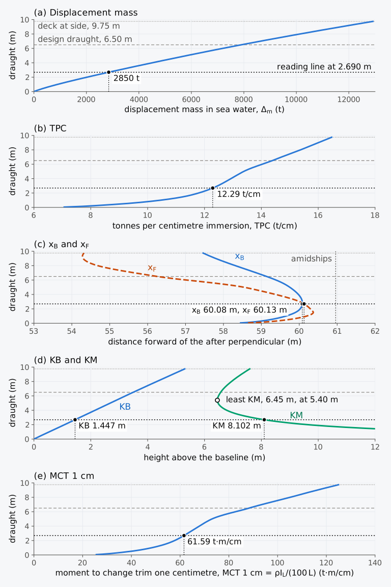
Figure 7.1 Hydrostatic curves of the Series 60 hull, upright and at even keel in sea water: (a) displacement mass; (b) TPC; (c) and ; (d) KB and KM; (e) MCT 1 cm. Each curve is read on the dotted line at 2.690 m, where the displacement mass is 2850 t.
Table 7.1 Hydrostatic values of the Series 60 hull, 121.92 m between perpendiculars and 16.256 m wide, upright and at even keel in sea water ( = 1.025 t/m³), moulded. and are measured forward of the AP, and amidships is at 60.96 m; MCT 1 cm is .
| (m) | (t) | TPC (t/cm) | (m) | (m) | MCT 1 cm (t·m/cm) |
|---|---|---|---|---|---|
| 1.0 | 895.9 | 10.44 | 59.65 | 60.20 | 48.38 |
| 2.0 | 2018.2 | 11.79 | 60.02 | 60.29 | 57.77 |
| 3.0 | 3233.7 | 12.46 | 60.08 | 60.01 | 63.08 |
| 4.0 | 4504.1 | 12.93 | 59.98 | 59.38 | 67.80 |
| 5.0 | 5819.2 | 13.38 | 59.75 | 58.55 | 73.08 |
| 6.0 | 7187.7 | 14.03 | 59.39 | 57.02 | 82.75 |
| 7.0 | 8625.5 | 14.71 | 58.87 | 55.65 | 93.54 |
| 8.0 | 10130.3 | 15.38 | 58.31 | 54.68 | 105.12 |
| 9.0 | 11699.5 | 16.00 | 57.79 | 54.30 | 116.17 |
Table 7.2 Heights of the centre of buoyancy and the metacentres, and the block coefficient, of the Series 60 hull at the draughts of Table 7.1. KM is KB + BM and is KB + , each summed before rounding. is based on the length between perpendiculars, the moulded breadth of 16.256 m and the draught.
| (m) | KB (m) | BM (m) | KM (m) | (m) | (m) | |
|---|---|---|---|---|---|---|
| 1.0 | 0.533 | 14.498 | 15.032 | 658.4 | 658.9 | 0.441 |
| 2.0 | 1.076 | 8.564 | 9.641 | 349.0 | 350.0 | 0.497 |
| 3.0 | 1.613 | 6.044 | 7.657 | 237.8 | 239.4 | 0.531 |
| 4.0 | 2.146 | 4.638 | 6.784 | 183.5 | 185.7 | 0.554 |
| 5.0 | 2.679 | 3.798 | 6.477 | 153.1 | 155.8 | 0.573 |
| 6.0 | 3.217 | 3.276 | 6.493 | 140.4 | 143.6 | 0.590 |
| 7.0 | 3.765 | 2.905 | 6.669 | 132.2 | 136.0 | 0.607 |
| 8.0 | 4.320 | 2.629 | 6.949 | 126.5 | 130.8 | 0.623 |
| 9.0 | 4.881 | 2.415 | 7.296 | 121.1 | 125.9 | 0.640 |
The shape of each curve follows from the form of the hull. The displacement grows faster than in proportion to the draught, because the waterplane widens as the ship sinks, and it rises by 100 TPC tonnes for each metre of draught. The TPC rises quickly near the keel, where the waterline leaves the flat of keel and climbs the turn of the bilge, and slowly between about 3 m and 5 m. Above 5 m it rises faster again, because the ends of the hull flare outwards. The centre of flotation is furthest forward at 1.5 m, 0.59 m aft of amidships, and lies less than 1 m aft of amidships between 1 m and 3 m. Above 1.5 m it moves aft, slowly at first and then quickly as the waterlines become fuller aft, to 4.71 m aft of amidships at 6.50 m. The centre of buoyancy follows it at a distance, because each new layer of volume is added at F. KB is almost a straight line, between and from 1 m upwards. KM is large at light draughts, where the volume is small for the breadth of the waterplane. It falls steeply as the volume grows faster than the second moment of the waterplane, reaches its least value of 6.45 m at 5.40 m and then rises slowly, as KB rises faster than BM falls. MCT 1 cm is proportional to , which grows as the waterline lengthens and fills out towards the ends.
7.1.3 Reading the curves
The curves are read at the draught of a level ship, or at the draught at the centre of flotation of a ship with a small trim. On a sheet of curves the values at one draught lie on one horizontal line. The line is drawn at the draught, and from each point where it crosses a curve a vertical leads down to the scale of that curve. For a known displacement the reader goes from the displacement scale to the displacement curve, and then along the horizontal line through that point9. Such a line is drawn in Fig. 7.1 at 2.690 m, the draught at which the Series 60 ship displaces 2850 t.
The curves of Fig. 7.1 are for sea water. In water of density , the displacement mass, the TPC and MCT 1 cm read at a draught are multiplied by , as in Chapter 3 for the displacement and the TPC. The volume, , , KB and KM are fixed by the immersed form and are read unchanged. A ship of known mass floats in that water at the draught at which the sea-water curves give .
In a table the values between two rows are found by linear interpolation, as in Chapters 3 and 6. That is accurate only where the curve between the rows is nearly straight.
Example 7.1. Reading the tables at a light draught. The Series 60 ship floats level in sea water at a displacement mass of 2850 t. Find its draught, TPC, , , KB, KM and MCT 1 cm by linear interpolation in Tables 7.1 and 7.2, where the rows at 2.0 m and 3.0 m give = 2018.2 t and 3233.7 t, TPC = 11.79 and 12.46 t/cm, = 60.02 and 60.08 m, = 60.29 and 60.01 m, KB = 1.076 and 1.613 m, KM = 9.641 and 7.657 m, and MCT 1 cm = 57.77 and 63.08 t·m/cm. Compare the results with the values of the curves of Fig. 7.1, which give a draught of 2.690 m and, there, TPC = 12.29 t/cm, = 60.08 m, = 60.13 m, KB = 1.447 m, KM = 8.102 m and MCT 1 cm = 61.59 t·m/cm.
7.2 Calculating the curves
7.2.1 From waterplanes to curves
A program that computes the curves begins with a series of waterlines, from the keel to the deck. For each it computes the properties of the waterplane: its area , the position of its centroid F, and its second moments about the centreline and about the transverse axis through F. Integrating the areas and their moments up the draught then gives the volume below each waterline and the centre of that volume,
each a running integral with a variable upper limit, evaluated at every waterline of the series as in Sec. 2.8.1. TPC, BM, KM, and MCT 1 cm then follow at each waterline from the expressions given above, and the coefficients of form from the volume, the areas and the main dimensions.
The volume can also be found the other way, by integrating the areas of the sections along the ship at each waterline. The sequence of calculations given by Hamlin5 does both: it takes the displacement and from the section areas, KB from the displacement curve and the waterplane quantities from the waterlines, and then integrates the waterplane areas up the draught as a check on the displacement and KB. Programs that work from a surface model or a mesh compute the quantities directly from it, and the relations between them are unchanged.
7.2.2 The spacing of the waterlines
In Sec. 2.8.1 the volume curve of the Series 60 hull was least accurate near the keel. There the waterplane area rises from 610 m² on the flat of keel, at first roughly as the square root of the height, and a parabola through waterplanes far apart cannot follow it. The remedy is to place the waterlines closer together where the waterplane changes fastest.
With seven waterplanes 1.083 m apart, from the keel to 6.50 m, Simpson’s rule gives a volume of 7677.6 m³ at 6.50 m, 0.36 % less than the 7705.7 m³ of the surface (Fig. 7.2(a)). At the design draught, 6.5024 m before it is rounded to 6.502 m, the surface holds 7709.1 m³, the 2.4 mm adding 1403 m² × 0.0024 m = 3.4 m³. On the evenly spaced waterplanes the first parabola gives too little area near the keel and too much at about 2 m. With seven waterplanes at 0, 0.25, 0.5, 1.5, 2.5, 4.5 and 6.5 m, and the rule applied to each pair of intervals with its own spacing, the volume is 7697.9 m³, 0.10 % less (Fig. 7.2(b)). KB comes out as 3.502 m and 3.494 m, against 3.490 m, although both integrations use seven waterplanes and differ only in their heights.
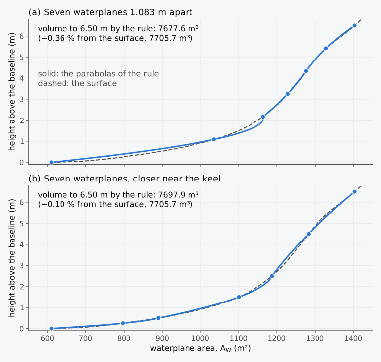
Figure 7.2 Waterplane area of the Series 60 hull against height, with seven waterplanes integrated by Simpson’s rule: (a) evenly spaced; (b) closer together near the keel.
A hydrostatics program uses many more waterlines. The curves of Fig. 7.1 are integrated on the heights at which the surface is defined, 0.8 to 1.8 cm apart and closest near the keel, and the error of the rule up the draught is then far below the precision of the tables.
7.2.3 Building the curves layer by layer
Equation (7.1) also shows how one row of a table follows from the row below it. Between two waterlines a layer of volume is added, with its moments about the AP and about the baseline. The new volume is the old volume plus the layer, and each new centre is the old centre and the centre of the layer combined in proportion to their volumes.
Example 7.2. From one row to the next. At a draught of 6.00 m the Series 60 hull has = 7012.4 m³, = 59.39 m and KB = 3.217 m. Its waterplanes at 6.00, 6.25 and 6.50 m have areas of 1369.2, 1386.9 and 1403.2 m², with their centres of flotation at 57.02, 56.61 and 56.25 m forward of the AP. Find , and KB at 6.50 m, using Simpson’s rule over the layer.
7.3 Relations between the curves
7.3.1 The slopes of the curves
The curves are not independent of one another. When the waterline rises by a small height , a layer of volume is added at the waterline, with its centroid at F6. The displacement therefore rises at the rate (Eq. (3.11)), which is 100 TPC per metre. Taking moments of the layer about the AP, the moment of the volume grows by . Since and ,
Taking moments of the layer about the baseline, where it lies at the height of the waterline,
where is the vertical prismatic coefficient of Eq. (1.15). Biran and López-Pulido derive the first forms of both relations6. Dividing Eq. (7.2) by Eq. (7.3) gives the direction in which B moves in the profile as the ship sinks,
7.3.2 The centre of buoyancy and the centre of flotation
By Eq. (7.2), B moves towards F as the ship sinks. When F lies forward of B, each new layer moves B forward, and when F lies aft of B, it moves B aft. Where F lies directly above B, stops changing. On curves drawn against a vertical draught, the curve of then has a vertical tangent6 where it crosses the curve of . On the Series 60 hull the crossing is at 2.82 m, where B lies 60.08 m forward of the AP, as far forward as it ever comes (Fig. 7.3(a)). Below that draught F lies forward of B and B moves forward, and above it F lies aft of B and B moves aft. The curves of some hulls never cross, and then moves in one direction only. In a hull that is symmetrical fore and aft, such as the box barge and the Wigley hull, and are both amidships at every draught and the two curves coincide.
By Eq. (7.3), KB always rises as the ship sinks, since the waterline is always above B. In a box = 1 and KB = , and KB rises at half the rate of the draught. When the waterplane grows with the draught, as it does in most ships, more of the volume lies high up, and KB rises faster than that. For the Series 60 hull at 6.50 m, with = 0.845, KB rises 0.548 m for each metre of draught.
Geometrically, Eq. (7.4) means that the line from B to F, drawn in the profile, is the tangent to the path that B follows as the waterline rises6. Figure 7.3(b) shows the path for the Series 60 hull and the lines from B to F at three draughts. At 2 m F lies 0.92 m above B and 0.27 m forward of it, and B moves up and slightly forward. At 7.5 m F lies far aft of B, and B moves aft and up along a line that points at F.
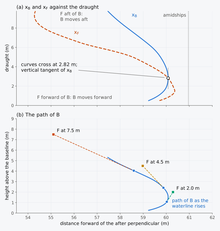
Figure 7.3 Centres of buoyancy and flotation of the Series 60 hull: (a) and against the draught; (b) the path of B, with the lines from B to F at 2.0, 4.5 and 7.5 m, the horizontal scale about twice the vertical.
Animation 7.1 shows the waterline rising on the Series 60 hull, with F on the waterline and B below it, and the two curves traced as the draught grows.
Animation 7.1 The waterline of the Series 60 hull rising from 0.30 m to 9.50 m. Above, the hull with F on the waterline and B below it, heights three times as large as lengths; below, xB (solid) and xF (dashed) traced against the draught. B moves forward while F lies forward of it, stops at 2.82 m, where the curves cross, and then moves aft. No sound; 9.8 s.
Predict 7.1. A barge of constant breadth has a flat bottom, a vertical stern and a bow raked forward, and its waterplane lengthens forward as it sinks. Decide whether its centre of buoyancy moves forward or aft as it is loaded.
7.3.3 Checking the curves
The relations of Sec. 7.3.1 were once used to check hand-drawn curves, and they still serve to find errors in curves that are plotted or copied outside the program that computed them6. For ordinary ship forms the curves are also fair, with few points of inflection, and unfairness usually points to an error in the input data or in the plotting5. A slope measured between two rows of a table can be compared with the slope that these relations give from the values at the middle row.
Example 7.3. Checking the curves at 6.50 m. The hydrostatic table of the Series 60 hull gives, at 6.4 m and 6.6 m, = 7754.9 t and 8042.5 t, = 59.19 m and 59.09 m, and KB = 3.435 m and 3.545 m. At 6.5 m, = 7705.7 m³, = 1403.2 m², = 56.25 m, = 59.14 m and KB = 3.490 m. Check the slopes of the three curves at 6.5 m against the relations between the curves.
7.4 Tank capacity and sounding tables
The contents of a tank are calculated in the way the volume of the hull is. The horizontal sections of the tank take the place of the waterplanes. Their areas, integrated up from the bottom of the tank, give the volume of liquid at each depth, and their moments give its centre5, as in Eq. (7.1). The relations of Sec. 7.3 hold for the tank as well. In particular, the volume of the contents rises with the depth of the liquid at the rate , the area of the free surface, as the volume of displacement rises at the rate . The second moment of each section about the longitudinal axis through its centroid, found as is found for a waterplane, is that of the free surface when the liquid stands at that height; multiplied by the density of the liquid, it gives the free surface moment of Chapter 5. The structure inside the tank is deducted from the moulded volume, usually as a percentage of it5.
On board, the contents of a tank are read from the ship’s calibration book, which tabulates the volume and the centre of gravity of the contents at heights 0.01 m to 0.20 m apart9. The level of the liquid is measured through a sounding pipe (Fig. 7.4(a)). A weighted tape or a rod is lowered down the pipe until it strikes a pad on the bottom of the tank, and the length wetted gives the sounding, the depth of the liquid measured from the bottom of the tank5,9. The ullage, the distance from the top of the sounding pipe or of an ullage plug down to the surface, is the reading advised for tanks of oil, which are usually filled to at most 98 % of their capacity to allow for expansion with heat; soundings are advised for tanks of water, which may be filled completely9. A sounding or an ullage is turned into a volume by reading the table at that level, as the hydrostatic table is read at a draught; in the tank of Fig. 7.4(b), a sounding of 1.60 m, or an ullage of 1.70 m, gives 117.6 m³. Where the pipe cannot reach the lowest point of the tank, the table often gives a considerable volume at a sounding of zero5. The IMO guidelines for the approval of stability instruments, MSC.1/Circ.1229, give as examples of the data stored in such an instrument the volume, the centre of the contents and the free surface moment of each compartment against the level of its contents10.
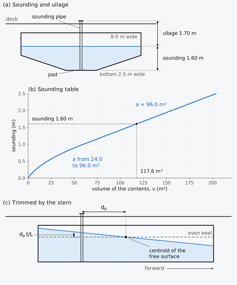
Figure 7.4 A sounding pipe in a fuel tank 12.0 m long: (a) transverse section through the pipe; (b) the sounding table of the tank as a curve; (c) longitudinal section in a ship trimmed by the stern, the trim exaggerated.
The table is computed for the ship at even keel, with the free surface parallel to the baseline. When the ship trims, the surface of the liquid stays level, and relative to the tank it turns, for a small trim, about the centroid of its own area, as the waterplane turns about F5. The depth of the liquid at that centroid is therefore unchanged, and the table read at that depth still gives the volume. A sounding pipe that does not pass through the centroid reads a different depth. With the pipe a distance aft of the centroid and the ship trimmed by by the stern, the liquid at the pipe is deeper than at the centroid (Fig. 7.4(c)). Since the volume rises at the rate with the depth, the volume read from the table for that sounding is too large by . The correction for a list5 has the transverse distance of the pipe from the centroid and in place of and .
7.5 Curves of hulls whose form changes abruptly
7.5.1 A casemate barge
The curves of an ordinary ship are smooth. Those of floating dry docks, offshore mobile platforms and integrated tug-barges may have corners at the draught where a large element of buoyancy goes under water or comes out of it. A vessel whose large compartments are sometimes flooded, such as a barge carrier with a dock that floods freely, needs a separate curve of a quantity for each condition. Such vessels need careful treatment5. A deck that goes under water is the simplest case.
Consider a barge 80 m long and 15 m wide, a box up to its deck at 6.00 m. Over the middle 50 m of its length stands a shield with vertical ends, whose sides rise from the deck edge at 36° to the horizontal to a flat roof 9.00 m above the keel and 6.74 m wide (Fig. 7.5). Forward and aft of the shield the deck is flat, so above 6.00 m only the shield cuts the water. The barge is an illustration of such a form, not a model of the Virginia.
Below the deck the barge is a box. Its waterplane is 1200 m², its TPC 12.30 t/cm, and at 6.00 m KB is 3.000 m, BM is m and KM is 6.125 m. As soon as the deck goes under, the waterplane is that of the shield, 50 m long and, at the deck edge, 15 m wide. Its area falls to 750 m² and its TPC to 7.69 t/cm. Its second moment about the centreline falls from 22,500 m⁴ to 14,062.5 m⁴, so BM falls to 1.953 m and KM to 4.953 m, with the displacement unchanged. MCT 1 cm falls from 82.0 to 20.0 t·m/cm, because the waterplane loses its ends, which contributed most to . Above the deck the shield narrows as the water rises, and the TPC and KM keep falling.
The displacement curve and the KB curve are continuous at the deck, since the volume does not jump, but their slopes change there, as Eqs. (3.11) and (7.3) require when jumps. The TPC, KM and MCT curves jump; Fig. 7.5 shows the first two. Interpolation in a table with no row at the deck, with rows at 5.5, 6.5 and 7.0 m, runs a straight line across the jump and gives a TPC of 9.64 t/cm at 6.00 m, a value the barge never has. A table for such a hull therefore needs two rows at the draught of the change, one just below it and one just above it, and a curve drawn through the rows must break there and not be faired across.
The jumps describe the barge upright and level. When it heels or trims, the deck edge or the deck ends cross the waterline at small angles, at a heel of 0.76° when the barge floats at 5.90 m or 6.10 m, and at a trim angle of only 0.143°, a total trim of 0.20 m over its 80 m length, since the deck ends lie 40 m from amidships. The waterplane then changes with the angle. The metacentric height and MCT 1 cm on either side of the jump therefore hold only at smaller inclinations than in an ordinary ship. At larger angles the righting lever depends on the whole inclined hull, and it does not jump.
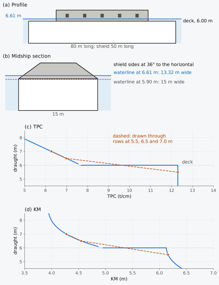
Figure 7.5 The casemate barge, 80 m by 15 m with its deck at 6.00 m: (a) profile, heights twice as large as lengths; (b) midship section, to scale; (c) TPC; (d) KM. Dashed: through the values at 5.5, 6.5 and 7.0 m, as from a table with no row at the deck.
Predict 7.2. The casemate barge floats at 5.90 m, with its deck 0.10 m above the water. Ballast is loaded at the height of its centre of gravity until it floats at 6.10 m, with the deck 0.10 m under water. Decide whether its metacentric height rises or falls, and roughly by how much.
Example 7.4. Ballast to bring the shield down. The casemate barge, 80 m long and 15 m wide, with its deck at 6.00 m and a shield 50 m long with vertical ends, whose sides slope at 36° to the horizontal from the deck edge, floats at 6.10 m in sea water. Find the ballast needed to bring the lower edge of the shield 0.61 m under water, and compare it with the ballast that the TPC of the hull below the deck, 12.30 t/cm, would suggest.
7.5.2 The Virginia
We can now return to the Virginia. It was meant to float with its deck under water at both ends and the lower edge of its shield 2 ft under water. The fighting waterline was therefore above the change of form, where only the shield cut the water and the waterplane was much smaller than that of the hull below. For the barge, the 0.61 m of water over the edge of the shield adds 442.7 t to the displacement mass, an average of 7.26 t/cm, while below the deck a mass of 442.7 t would change the draught by only 36 cm. A ship floating at such a waterline rises quickly as coal and stores are used, and the shield comes out of the water sooner than the TPC of the hull below the deck would suggest. This agrees with what Jones recorded on the second day of the fight, when the lower edge of the shield forward had come up to the water3.
For a ship designed to float above such a change of form, a small error in the calculated weight is a large error in the draught, and the Virginia rode too high until ballast brought it down. In May the change of form worked the other way. Once the deck and the lower edge of the shield were out of the water, the waterplane was that of the whole hull, and each further tonne thrown overboard lifted the ship less than before. The stability of such a ship also changes at that draught. In the barge, KM is 1.65 m higher with the deck just out of the water than with the edge of the shield 0.61 m under, so lightening the barge changes its metacentric height as well as its draught.
A vessel designed to float on a small waterplane is sensitive to weight in this way at its operating draughts. A SWATH, a small-waterplane-area twin hull, carries most of its displacement in two hulls well below the surface and pierces the surface only with thin struts11. A harbour surveillance craft of 95 t, compared as a SWATH and as a conventional ship of equal displacement, has a waterplane of 22 m² in the first form and 120 m² in the second11. Its TPC in sea water is therefore 0.23 t/cm as a SWATH and 1.23 t/cm as a conventional ship, and an error of 1 t in its weight changes the draught by 4.4 cm against 0.8 cm. Weight control is one of the main concerns in designing such craft11.
7.5.3 Exploring the curves (Explorer 7.1)
Explorer 7.1 draws the curves of the four hulls of this chapter: the box barge 60 m long and 12 m wide, the Wigley hull, the Series 60 hull and the casemate barge. The curves of the box barge, the Wigley hull and the casemate barge come from their formulas, and those of the Series 60 hull from the calculation of Fig. 7.1. Choose a hull and a quantity, then move the draught to read its values. The box barge shows the simplest curves, and the casemate barge the jumps at its deck. MCT 1 cm is for every hull, as in Table 7.1.
7.6 Approximate curves for early design
7.6.1 Formulas for KB
Before the lines of a hull exist, a designer may need KB at a given draught from the displacement and the waterplane area. Morrish’s formula, Eq. (4.9), replaces the curve of waterplane area by a figure of straight lines through its ends that encloses an equal area, and gives . Posdunine’s formula, , also uses only these two quantities. Morrish’s formula is close for ships of ordinary form, at light draughts as well as at the load draught, and Posdunine’s agrees particularly well for ships with a high midship coefficient5. Divided by the draught, both depend on the hull only through its vertical prismatic coefficient :
Posdunine’s formula is exact for any body whose waterplane area grows as a power of the height above the keel, . The volume is then , which gives , and its moment about the keel is , so that . The box () and the wedge () are such bodies, and so is a prism with parabolic sections whose vertex is at the keel (), for which KB is . Of these bodies, Morrish’s formula is exact only for the box and the wedge, and for the parabolic prism it gives . Between = 1/2, the wedge, and 1, the box, Morrish’s value is never below Posdunine’s, and it exceeds it by at most , at . No formula that depends only on can be exact for every hull. The Wigley hull at its design draught has = 2/3, as the parabolic prism has, but its KB is .
In Fig. 7.6 the two formulas are compared with the integrated KB of the Wigley hull, whose midship coefficient is 0.67 at its design draught, and of the Series 60 hull, whose midship coefficient there is 0.97. Since Morrish’s value is the higher of the two, Morrish’s formula is the closer on a hull whose KB lies above both, and Posdunine’s on a hull whose KB lies below both. For these two hulls the shape of the sections explains which case each is in. The broad flat of bottom of the Series 60 hull gives it waterplane area near the keel, which places its volume, and KB, low for its : its TPC just above the keel is about 7 t/cm, half its value at the design draught. The parabolic sections of the Wigley hull give no waterplane at the keel, and its KB lies high for its . The midship coefficient is a sign of this, not a rule: it describes one section, while KB depends on how the waterplane area of the whole hull grows with the height above the keel. On the Wigley hull both formulas are low, and Morrish’s is the better. At the design draught of 6.25 m it gives 3.819 m against 3.906 m, 8.7 cm low, and Posdunine’s gives 3.750 m, 15.6 cm low. On the Series 60 hull at 6.50 m both are high, and Posdunine’s is the better. It gives 3.523 m against 3.490 m, about 3.4 cm high, and Morrish’s gives 3.586 m, 9.6 cm high. Below 5 m Posdunine’s formula stays within 1 cm of the Series 60 curve, but once the hull is defined the integrated value is used instead of either.
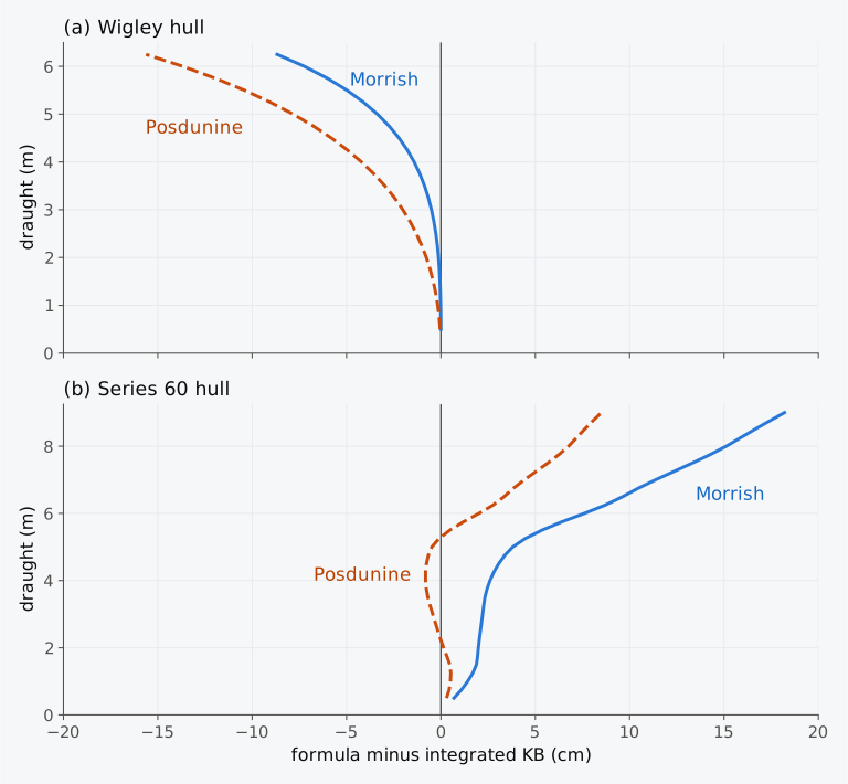
Figure 7.6 Error of the formulas of Morrish and Posdunine against the integrated KB of (a) the Wigley hull and (b) the Series 60 hull. A positive error places B too high.
7.6.2 An estimate of MCT 1 cm
MCT 1 cm can also be estimated from quantities known early in a design. With the waterplane-area coefficient and the longitudinal inertia coefficient of Sec. 2.5.2, the TPC is and is . The length cancels between the two, and
with the TPC in t/cm, in m and in t/m³. For a rectangular waterplane , and = 8.13 in sea water. For the parabolic waterplanes of the Wigley hull = 0.4 and = 2/3, and = 7.32. A formula due to Normand, published in 1882, estimates from the area of the waterplane8, . It amounts to taking , and so = 7.17 in sea water. Kemp and Young give = 7.2 for general cargo ships and 7.8 for oil tankers12. These are estimates for early design, and their accuracy for a new hull is not assured. With = 7.17 the estimate is 12 % low for a box and 2 % low for the Wigley hull at its design draught. For the Series 60 hull at 6.50 m it gives t·m/cm, 3.3 % above the 88.27 t·m/cm of the curve, and over the draughts of Table 7.1 the constant of this hull varies between about 6.6 and 7.4. Such an estimate serves early in a design and as a check on a calculated curve8.
7.6.3 Hulls derived by stretching
A new hull is often derived from a successful parent by stretching its offsets by factors , and along the length, the breadth and the height. The coefficients of form are unchanged by such a stretch, and the hydrostatic curves change in a simple way6. The waterplane of the new hull at the draught is the parent’s waterplane at , stretched by and , and the volume below it is the parent’s volume stretched by all three factors. Every curve of the new hull therefore follows from the parent’s at the corresponding draught:
the last with the density of the water unchanged. The TPC scales as . BM scales as because grows with the cube of the breadth and the first power of the length, and the volume with all three. MCT 1 cm, taken as , scales as . The moment of a loaded ship, , adds , which scales as when KG scales with the depth. Programs find the curves of a hull stretched in this way, an affine hull, by changing the scale factors only6.
Example 7.5. A longer and wider Series 60 hull. A new design is derived from the Series 60 hull by stretching its lengths by 1.10 and its breadths by 1.05, with its heights unchanged. At a draught of 6.50 m the parent has = 7705.7 m³, TPC = 14.38 t/cm, = 59.14 m, = 56.25 m, KB = 3.490 m, BM = 3.078 m, = 136.3 m and MCT 1 cm = 88.27 t·m/cm in sea water. Find the corresponding values for the new hull at 6.50 m, with its KM and displacement mass.
7.7 Hydrostatics of a trimmed ship
7.7.1 Bonjean curves at a trimmed waterline
The hydrostatic curves of Sec. 7.1 describe the ship at even keel, and we will call them the level curves. For a moderate trim, the displacement is read from them at the draught at F and corrected by the second trim correction, tonnes (Eq. (6.13)). The correction needs MCT 1 cm as , a property of the waterplane, so the approximation of Sec. 7.1 does not enter it. Moore recommends evaluating the buoyancy and its centre directly from the hull at the trimmed waterline, and allows the level curves only for a moderate trim with no abrupt change of the waterplane between the trimmed and the level waterlines7. The limit of a trim of about 1/150 of the length7, 0.81 m for the Series 60 ship, applies to draughts found from the level curves (Sec. 6.5.2), not to the displacement at a known waterline.
In a calculation by hand, the volume at the trimmed waterline is found from the Bonjean curves. The Bonjean curve of the section at gives its immersed area up to any height , and with it the moment of that area about the baseline (Eqs. (1.23) and (1.24)). At a straight waterline that crosses the section at the height ,
where and KB are in the ship’s axes5,6. The integrals run between the perpendiculars, and a part of the hull beyond them is added separately when it is immersed. In this chapter “the whole hull” means the surface itself integrated below the trimmed waterline, with its ends beyond the perpendiculars.
Figure 7.7 shows the Bonjean curves of the Series 60 hull at every second station, drawn from their station lines on the profile, with the waterline of the ship after all its cargo has been discharged. The section areas and moments read where this waterline crosses the curves are listed in Table 7.3.
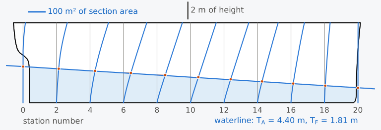
Figure 7.7 Bonjean curves of the Series 60 hull at stations 0 to 20, every second station, with the waterline = 4.40 m, = 1.81 m. The dots mark the section areas below the waterline.
Table 7.3 Section areas and their moments about the baseline below the waterline = 4.40 m, = 1.81 m, read from the Bonjean curves of the Series 60 hull, with Simpson’s multipliers .
| Station | (m) | (m) | (m²) | (m³) | |
|---|---|---|---|---|---|
| 0 | 0.000 | 4.400 | 0.00 | 0.0 | 1 |
| 2 | 12.192 | 4.141 | 13.18 | 31.1 | 4 |
| 4 | 24.384 | 3.882 | 30.74 | 66.6 | 2 |
| 6 | 36.576 | 3.623 | 44.66 | 87.7 | 4 |
| 8 | 48.768 | 3.364 | 49.80 | 88.1 | 2 |
| 10 | 60.960 | 3.105 | 47.74 | 76.8 | 4 |
| 12 | 73.152 | 2.846 | 40.39 | 60.6 | 2 |
| 14 | 85.344 | 2.587 | 27.51 | 38.9 | 4 |
| 16 | 97.536 | 2.328 | 13.53 | 18.0 | 2 |
| 18 | 109.728 | 2.069 | 4.68 | 5.6 | 4 |
| 20 | 121.920 | 1.810 | 0.00 | 0.0 | 1 |
Example 7.6. Displacement at a large trim. After discharging all its cargo, the Series 60 ship floats at = 4.40 m and = 1.81 m, a trim of 2.59 m by the stern. Table 7.3 gives the section areas and their moments about the baseline, read from the ship’s Bonjean curves where this waterline crosses stations 0 to 20 at every second station, 12.192 m apart. (a) Find , , and KB by Simpson’s rule. (b) At the mean of the end draughts, 3.105 m, the level curves give = 59.96 m, and at the draught at F they give = 3391.2 t. MCT 1 cm is 61.27 t·m/cm half a metre below that draught and 66.03 t·m/cm half a metre above it. Find the displacement mass from the level curves, with and without the second trim correction. (c) Compare both results with the whole hull, which displaces 3323.4 m³ at this waterline, with = 55.17 m.
7.7.2 Displacement against trim
Figure 7.8 shows how the displacement of the Series 60 ship changes as it trims about a fixed draught at F of 6.00 m, from 4 m by the head to 4 m by the stern. The level curves give 7187.7 t at every trim. The whole hull displaces more at any trim, 64.6 t more at 4 m by the head and 70.5 t more at 4 m by the stern, because the immersed end gains more volume than the emerged end loses. The second trim correction follows the hull to within about 8 t by the head and 2 t by the stern. The Bonjean curves at 21 stations follow it within 2.6 t, except at the largest trim by the stern. Since they stop at the perpendiculars, they leave out the overhang of the stern aft of the AP, which a trim by the stern immerses. At 4 m by the stern, with the aft draught at 7.87 m, that overhang displaces 5.8 t.
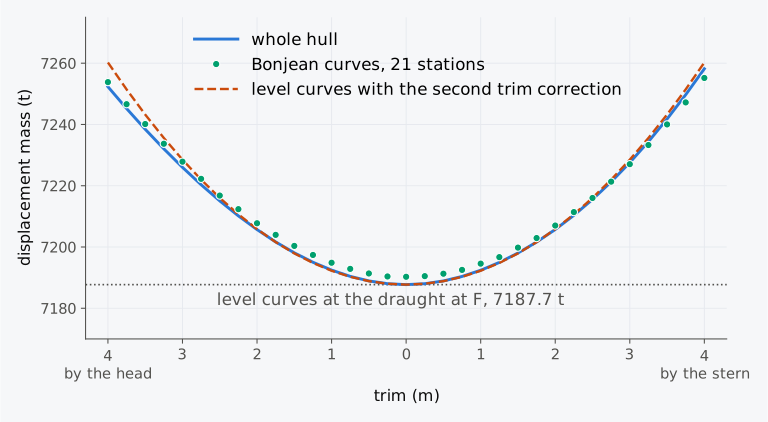
Figure 7.8 Displacement of the Series 60 ship against trim at a constant draught at F of 6.00 m: the whole hull; Simpson’s rule over the Bonjean curves at 21 stations; the level curves with and without the second trim correction.
When the effect of trim on displacement is of unusual importance, curves of trim corrections may be calculated for a series of trimmed waterlines, for example at trims of 1 m and 2 m by the head and by the stern, at a series of draughts5. The Bonjean curves make such calculations easier. The corrections found in this way are more accurate than those from the curve of change of displacement for one centimetre of trim, because they do not assume that the ship is wall-sided at the waterline5. When the calculation is made by computer, the Bonjean curves can still be used but rarely are7.
7.7.3 Bonjean calculator (Calculator 7.1)
Calculator 7.1 finds the displacement, and KB of the Series 60 ship at a straight waterline, given the draughts at the perpendiculars. It reads the Bonjean curves of the Series 60 hull, tabulated every 0.05 m of height, at 11 or 21 stations, applies Simpson’s rule as in Example 7.6 and shows each step. For comparison it gives the values of the whole hull at the given draughts, interpolated in a table computed on the surface. The locked presets repeat Example 7.6 at 11 and at 21 stations, and “Your own waterline” accepts any draughts between 0.50 m and 9.50 m with a trim of up to 6 m.
7.8 Hydrostatic curves in industry today
This section describes practice in 2026.
The stability booklet. Among the contents that the International Code on Intact Stability, 2008 (IS Code), recommends for a stability booklet are hydrostatic curves or tables and cross curves of stability, which give the lever KN of the heeled ship against its displacement at a series of angles of heel. Both are to cover the ranges of displacement and trim expected in normal operation, and the cross curves are to be calculated on a free-trimming basis, with the ship free to trim as it heels6,13. The Code also recommends including a sounding table for each tank, with its capacities, centres of gravity and free surface data13. The calculations are to include the volume up to the upper surface of any deck sheathing, and the appendages and sea chests are to be considered13. The stability booklet of the bulk carrier Armia Krajowa, for example, gives its even-keel hydrostatic tables every 0.5 m of draught and further tables at three trims, of 1, 2 and 3 m by the stern14. Wawrzyński computed the displacement of the trimmed ship from its Bonjean scale, a table of section areas against draught, as a reference for the corrections of a draught survey14.
Stability instruments. Under the IS Code, an approved stability instrument either works from the hydrostatic and stability data of the approved booklet, stored in the program, or computes them from a model of the hull form13. In the first case the stored data must be reproduced exactly. Differences that come from using hydrostatic data for trims other than those in the booklet may be accepted after review by the Administration13. MSC.1/Circ.1229 and the unified requirement of the classification societies for such software, IACS UR L5, give as examples of the hydrostatic data that a program holds the displacement, LCB, LCF, VCB, KMt and MCT against draught10,15. These are the displacement, , , KB, KM and MCT 1 cm of this chapter. A table against draught alone holds MCT 1 cm either as , which needs no height of G7, or computed with an assumed standard height of G5. A program that computes from a model of the hull form must agree with the approved data within the tolerances10 of MSC.1/Circ.1229, given in Sec. 2.10.2. Loading software uses table look-up and interpolation in the hydrostatic tables, or computes directly from the hull model, and often replaces the TPC by the derivative of the displacement with respect to the draught7. Programs compute the curves from a surface model or a mesh of the hull by the methods of Sec. 2.10.1, and the hull passes between programs in the formats of Sec. 1.9.2.
The inclining experiment. The hydrostatic data are also the starting point of the inclining experiment, from which the lightship centre of gravity is found. The IS Code asks that the actual trim of the ship and, where practical, the deflection of its keel be taken into account in the hydrostatic data. Because the waterplane can change markedly as the ship heels, the hydrostatic data for the actual trim and the largest expected angles of heel are to be checked before the test13. The hydrostatic curves or data are among the plans that the person in charge of the test must have at hand13.
Stability in waves. A wave of a length comparable to the ship’s changes the waterplane as it passes16. IMO’s interim guidelines on the second generation intact stability criteria, MSC.1/Circ.1627 of December 2020, issued for trial use beside the mandatory criteria of the IS Code, assess five modes of stability failure in waves17. Among them are parametric roll and pure loss of stability, the loss of righting lever while a wave crest stays amidships16. For both, the first level of assessment reads upright hydrostatic data at draughts other than the loading draught, and the data may be those for even keel16,17. For pure loss of stability, GM is recalculated with the transverse second moment of a level waterplane lowered by half the height of a wave as long as the ship and of steepness 0.0334, the ratio of its height to its length, in place of the second moment at the loading draught16,17. For parametric roll, the amplitude of the variation of GM is the difference between the second moments of level waterplanes raised and lowered by half the height of a wave also as long as the ship and of steepness 0.0167, divided by twice the volume of displacement16,17. The waterplanes are not lowered below a quarter of the draught of the fully loaded departure condition nor raised above the moulded depth, and both checks also need the volume of displacement up to that depth on even keel, so the curves must reach the deck17.
7.9 From hydrostatic curves to stability at large angles
The hydrostatic curves describe the ship upright, in waterplanes parallel to its baseline, and supply the hull data for initial stability in that condition. KM is read from the curves at the draught and KG comes from the weight table. Their difference, with the free-surface correction where needed, is the fluid GM (Sec. 5.3) that governs the righting moment at small angles of heel. At larger angles the waterplane is inclined to the baseline and its shape changes with the angle. The deck edge or the bilge may cross it, much as the deck of the casemate barge crossed its waterline. The upright curves cannot show this, because their values at a draught depend only on the hull below that waterline: a higher deck on the Series 60 hull would leave every value in Tables 7.1 and 7.2 unchanged, yet it would keep the deck edge out of the water to a larger angle of heel. The wider hull of Example 7.5 gains 0.315 m of KM but brings its deck edge to the water at a smaller angle. In Chapter 8 we will compute the hydrostatics of the heeled ship at every angle and displacement as the cross curves of stability, which give KN, the large-angle counterpart of KM. Like KM, KN depends only on the hull at a given trim, and it is computed in advance for a range of displacements. Combined with the KG of the weight table, as KM is, it gives the righting lever of a loaded ship at large angles of heel.
Summary
- The hydrostatic curves give the hydrostatic properties of the hull at every draught, upright and at even keel: the displacement, TPC, , , KB, KM, , , MCT 1 cm and the coefficients of form. They are fixed by the form of the hull and the density of the water for which they are drawn, and the loading decides only the draught at which they are read.
- The curves are computed from waterplanes at a series of waterlines, whose areas and moments are integrated up the draught, Eq. (7.1). The waterlines must be closer together where the waterplane changes fastest, near the keel.
- On a sheet the curves are read along a horizontal line at the draught. In water of density the displacement mass, the TPC and MCT 1 cm of sea-water curves are multiplied by , and the volume, the centres, KB and KM are read unchanged. A table is read by linear interpolation only between rows close enough for the curve to be nearly straight between them. KM, which bends strongly at light draughts, needs the closest rows.
- The slopes of the curves are related: , and . B always moves towards F as the ship sinks, is stationary where the curves of and cross, and the line from B to F is the tangent to the path of B.
- These relations, and the fairness of the curves, are checks on calculated or plotted curves.
- The capacity table of a tank is computed in the way the displacement curve is, and the volume of the contents rises with their depth at the rate , the area of the free surface. On board the table is read at a sounding, the depth of the liquid above the bottom of the tank, or at an ullage, the distance from the top of the sounding pipe down to the surface. In a ship trimmed by by the stern, a sounding taken a distance aft of the centroid of the free surface overstates the volume by .
- Where the form changes abruptly, as when a deck goes under water, TPC, KM and MCT 1 cm jump and the displacement and KB curves have corners. A table needs rows just below and just above that draught, and the curves must not be faired across it.
- Morrish’s and Posdunine’s formulas, Eq. (7.5), estimate KB/ from the vertical prismatic coefficient only. Posdunine’s is exact when the waterplane area grows as a power of the height. For between 1/2 and 1 Morrish’s value is never the lower of the two, so Morrish’s did better on the Wigley hull, whose KB lies above both, and Posdunine’s on the Series 60 hull at 6.50 m, whose KB lies below both.
- MCT 1 cm, taken as , can be estimated as , with = 8.13 for a rectangular waterplane and 7.17 by Normand’s formula for , both in sea water.
- A hull stretched by , and has curves that follow from its parent’s by Eq. (7.6), with BM scaling as and MCT 1 cm, taken as , as .
- At a large trim the displacement and centre of buoyancy are found directly from the hull at the trimmed waterline, or from the Bonjean curves along it, Eq. (7.7), with any immersed part beyond the perpendiculars added. The level curves at the draught at F with the second trim correction come close at moderate trims.
Notes on the data
The Virginia. Its dimensions, draughts and history are from the accounts of three of its officers, Ramsay2, Jones3 and Newton1, and from Quarstein4. The accounts differ in detail. Newton gives the shield as about 160 ft (48.8 m) long and 22 in (0.56 m) thick, with its sides at 35°, and the submerged ends as about 58 ft (17.7 m) each1, where Ramsay gives about 180 ft (54.9 m), 2 ft (0.61 m), 36° and 50 ft (15.2 m). Ramsay gives its draught in the battle as 23 ft (7.01 m), and Jones as over 22 ft (6.71 m) before its refit and 23 ft after it. Its lines are not used in this chapter.
The casemate barge. The barge of Sec. 7.5 is illustrative. Its slope of 36° echoes that of the Virginia, but its other dimensions are chosen for clarity and are not the ship’s. Its curves are found from its formulas, given in scripts/ch07_data.py, in sea water.
The curves of the Series 60 hull. The curves are computed by scripts/ch07_data.py on the Series 60 surface of Chapter 1, by integration on the heights at which the surface is defined, with MCT 1 cm from , the -based approximation of Sec. 7.1. The values are moulded and in sea water of density 1.025 t/m³, without the shell or appendages. Tables 7.1 and 7.2 and Figs. 7.1 to 7.3 show them. The waterplanes of Example 7.2 are those of the Series 60 surface. The tables printed in Chapters 3 and 6 are rows of these curves.
The tank of Fig. 7.4. It is the fuel tank of Exercise 7.17, 12.0 m long, 2.0 m wide at the bottom and 8.0 m wide from 1.0 m up, with its sounding pipe 3.0 m aft of the middle. The top of the tank at 2.50 m, the deck at 3.10 m and the top of the pipe at 3.30 m above the bottom are chosen for the figure, and the pipe is drawn wider than a real one. In panel (c) the surface is drawn at a slope of 1 in 10 to the bottom of the tank, far steeper than any trim in the text, to make the difference in depth at the pipe visible.
The Bonjean curves and the trimmed hull. The Bonjean curves of the Series 60 hull are tabulated every 0.05 m at stations 0 to 20, between the perpendiculars, and read by linear interpolation in height. “The whole hull” means the surface integrated below the trimmed waterline, including the parts aft of the AP and forward of the FP, by the method of Chapter 3 (ch03/scripts/inclined.py). The waterline of Example 7.6 is that of the discharged condition of Chapter 6, solved on the hull as 4.399 m aft and 1.812 m forward and rounded here to 4.40 m and 1.81 m.
The trims in the tables of the Armia Krajowa. Wawrzyński14 gives them as −1, −2 and −3 m. They are read here as trims by the stern, as they are when trim is taken as the forward draught less the aft draught.
Explorer 7.1 and Calculator 7.1. The explorer reads tables written by scripts/ch07_data.py, every 0.1 m of draught: from their formulas for the box barge, the Wigley hull and the casemate barge, and from the integration described above for the Series 60 hull. The table of the casemate barge has two rows at the deck, one just below it and one just above it. The calculator reads the tabulated Bonjean curves, rounds each area and moment half up to 0.01 m² and 0.1 m³, and rounds each product to the digits shown, so that the columns add up to the printed sums. For comparison it gives the whole hull, integrated at draughts every 0.25 m from 0.50 m to 9.50 m at each end and interpolated by parabolas through the three nearest draughts at each end.
Exercises
Under each exercise, “Show answers” opens its short answers and “Show full solution” its worked solution. Unless stated otherwise the water is sea water of density 1.025 t/m³ and the draughts are moulded.
7.1 The Series 60 ship floats level at a displacement mass of 6000 t. Using Tables 7.1 and 7.2, find its draught, TPC, , , KB, KM and MCT 1 cm by linear interpolation.
7.2 In Example 7.1, linear interpolation between the rows at 2.0 m and 3.0 m gave KM = 8.284 m for the Series 60 ship at 2850 t, while the curves give 8.102 m at the draught of 2.690 m. Fit a parabola through the values of KM at 2.0, 3.0 and 4.0 m, 9.641, 7.657 and 6.784 m, and find KM at 2.690 m.
7.3 A box barge 60 m long and 12 m wide floats in sea water. (a) Show that its TPC and MCT 1 cm, taken as , do not change with the draught, and find them. (b) Find its displacement mass, KB, BM and KM at a draught of 3.00 m.
7.4 The half-breadth of the Wigley hull, 100 m long and 10 m wide, with a design draught = 6.25 m, is , with and . Show that the area of its waterplane at the height is , and integrate it to find and KB. Evaluate , TPC, and KB at a draught of 4.00 m.
7.5 At a draught of 5.00 m the Series 60 hull has = 5677.3 m³, = 59.75 m and KB = 2.679 m. Its waterplanes at 5.00, 5.25 and 5.50 m have areas of 1305.3, 1318.7 and 1334.1 m², with their centres of flotation at 58.55, 58.25 and 57.89 m forward of the AP. Find , and KB at 5.50 m.
7.6 Show that, when a ship whose centre of flotation lies a distance aft of amidships trims 1 cm by the stern at a constant draught amidships, its displacement increases by tonnes. Evaluate this change for the Series 60 ship at 2.0, 4.0 and 6.0 m, where Table 7.1 gives TPC = 11.79, 12.93 and 14.03 t/cm and = 60.29, 59.38 and 57.02 m.
7.7 The hydrostatic table of the Series 60 hull gives = 3109.3 t and 3358.6 t and KB = 1.560 m and 1.667 m at 2.9 m and 3.1 m. At 3.0 m it gives = 3154.8 m³, = 1216.1 m², KB = 1.613 m, = 60.08 m and = 60.01 m. Check the slopes of the displacement and KB curves at 3.0 m against Eqs. (3.11) and (7.3), and find the slope of the curve of there.
7.8 Use Eq. (7.3) to find the rate at which KB rises with the draught for a box and for the Wigley hull at its design draught of 6.25 m, where = 2/3 and KB = 3.906 m. Confirm the second value by differentiating the expression for KB found in Exercise 7.4.
7.9 At 2.0 m the Series 60 hull has = 1969.0 m³, = 1150.3 m², = 60.29 m and = 60.02 m. Use Eq. (7.2) to estimate at 2.5 m, and explain why the estimate exceeds the value of 60.07 m that the curves give there.
7.10 The casemate barge of Sec. 7.5, 80 m long and 15 m wide, has its deck at 6.00 m and a shield 50 m long with vertical ends, whose sides slope inwards at 36° to the horizontal from the deck edge. Its centre of gravity is 4.20 m above the keel. Find its metacentric height at draughts of 5.90 m and 6.61 m.
7.11 A casemate barge 80 m long and 15 m wide, a box up to its deck at 6.00 m, carries over the middle 50 m of its length a shield whose sides rise from the deck edge. Find the slopes of its displacement curve and of its KB curve in sea water just below and just above the deck.
7.12 At 5.00 m the Series 60 hull has = 5677.3 m³ and = 1305.3 m², and its integrated KB is 2.679 m. Estimate KB by Morrish’s and Posdunine’s formulas, and find the error of each.
7.13 Using the expressions of Exercise 7.4, find , and KB of the Wigley hull, 100 m long and 10 m wide, at half its design draught of 6.25 m, that is at 3.125 m, and estimate KB there by Morrish’s and Posdunine’s formulas.
7.14 A second design is derived from the Series 60 hull by stretching its breadths and heights by 1.10, with its lengths unchanged. At 6.50 m the parent has = 7705.7 m³, TPC = 14.38 t/cm, KB = 3.490 m, BM = 3.078 m, = 136.3 m and MCT 1 cm = 88.27 t·m/cm. Find the corresponding draught of the new hull and, there, its displacement mass, TPC, KB, BM, KM, and MCT 1 cm.
7.15 The Series 60 ship floats at = 5.00 m and = 7.00 m, a trim of 2.00 m by the head. Where this waterline crosses stations 0 to 20 at every second station, 12.192 m apart, the ship’s Bonjean curves give section areas of 0.00, 18.48, 48.21, 74.68, 89.35, 94.80, 93.56, 78.18, 49.95, 20.89 and 0.01 m². Find , and by Simpson’s rule, and compare the volume with that of the whole hull, 6943.8 m³.
7.16 The Series 60 ship floats with a draught at F of 6.00 m and a trim of 3.00 m by the stern. The level curves give = 7187.7 t at 6.00 m, and MCT 1 cm = 77.22 t·m/cm at 5.50 m and 88.27 t·m/cm at 6.50 m. Estimate its displacement mass with the second trim correction, and compare it with the whole hull, 7227.6 t, and the Bonjean curves at 21 stations, 7227.0 t.
7.17 A fuel tank 12.0 m long has vertical ends and a uniform transverse section, 2.0 m wide at the bottom of the tank, which widens linearly to 8.0 m at 1.0 m above the bottom and has vertical sides above that. (a) Find the volume in the tank and the height of the centre of the contents above the bottom of the tank at soundings of 1.00 m and 2.00 m. (b) The sounding pipe is 3.0 m aft of the middle of the tank. The Series 60 ship, 121.92 m between perpendiculars, trims 2.00 m by the stern, and the pipe reads 2.00 m. Find the volume in the tank.
Symbols introduced in this chapter
Symbols defined in earlier chapters, among them , , , , , KB, BM, KM, KN, , TPC, MCT 1 cm, , , , , , the interval of an integration rule and the coordinates and of the Wigley hull, keep their meaning.
| Symbol | Meaning | Unit |
|---|---|---|
| fraction of the interval between two rows of a table | – | |
| volume of a layer between two waterlines | m³ | |
| , | moments of that layer about the AP and about the baseline | m⁴ |
| volume of liquid in a tank | m³ | |
| area of the free surface of the liquid in a tank | m² | |
| distance of a sounding pipe aft of the centroid of the free surface | m | |
| , | breadth of the shield of the casemate barge at a height above its deck | m |
| , | coefficient and exponent of a waterplane area that grows as a power of the height, | m2−n, – |
| constant of the estimate , with TPC in t/cm and in m | m²·cm/t | |
| , , | factors by which a hull is stretched along its length, breadth and height | – |
| , , … | quantities of a stretched hull | as unstretched |
| height of a trimmed waterline at the section at | m | |
| Simpson’s multiplier | – | |
| design draught of the Wigley hull, 6.25 m | m | |
| draught of the Wigley hull as a fraction of its design draught | – |
Corrections
Corrections to version 1.0, released on 3 November 2026, with their dates.
- 5 November 2026. Sec. 7.6.1 gives the estimates of KB at 6.50 m to the millimetre, as the printed inputs give them: 3.523 m by Posdunine’s formula and 3.586 m by Morrish’s, in place of 3.5861 m, against 3.490 m.
- 5 November 2026. Table 7.2 gives the height of the longitudinal metacentre, , which Sec. 7.1.1 and the closing sections of Chapters 4 and 6 name among the curves.
- 5 November 2026. Sec. 7.9 calls the GM corrected for free surfaces the fluid GM, in place of the effective GM, a term that Chapter 13 uses for a supported ship. The route for a first reading says which outcomes and later chapters need Secs. 7.6 and 7.7, and Sec. 7.5.1 says which curves Fig. 7.5 shows.
- 6 November 2026. Sec. 7.1.1 is headed “Quantities in the hydrostatic curves”, in place of “What the curves contain”. Its text is unchanged.
References
- Newton, V. (1892). The Confederate States ram Merrimac or Virginia: The history of her plan & construction and her engagements with the United States fleet, March 8–9, 1862 (Reprinted from the Southern Historical Society Papers, Vol. 20). Wm. Ellis Jones. Retrieved October 11, 2026, from https://community.village.virginia.edu/nauletters/node/10744 Cited: ↑ · ↑ · ↑ · ↑ · ↑ · ↑
- Ramsay, H. A. (1912). The Merrimac and the Monitor. In J. L. Worden, S. D. Greene, & H. A. Ramsay, The Monitor and the Merrimac: Both sides of the story (ch. II). Harper & Brothers. (Public domain; Project Gutenberg eBook No. 24612.) Retrieved October 11, 2026, from https://www.gutenberg.org/ebooks/24612 Cited: ↑ · ↑ · ↑ · ↑
- Jones, C. ap R. (1883). Services of the Virginia (Merrimac). Southern Historical Society Papers, 11, 65–74. Retrieved October 11, 2026, from https://navyandmarine.org/ondeck/1862services_of_virginia.htm Cited: ↑ · ↑ · ↑ · ↑ · ↑ · ↑ · ↑
- Quarstein, J. V. (2012). Proving the power of iron over wood. Naval History, 26(2). Retrieved October 11, 2026, from https://www.usni.org/magazines/naval-history-magazine/2012/april/proving-power-iron-over-wood Cited: ↑ · ↑ · ↑
- Hamlin, N. A. (1988). Ship geometry. In E. V. Lewis (Ed.), Principles of naval architecture: Vol. I. Stability and strength (2nd rev., Chapter I). Society of Naval Architects and Marine Engineers. Cited: ↑ Section 5.1 · ↑ Section 5.1 · ↑ Sections 5.11 and 5.15 · ↑ Section 5.12 · ↑ Section 5.1 · ↑ Sections 5.1 and 5.15 · ↑ Sections 5.6 and 5.13 · ↑ Section 5.1 · ↑ Section 5.15 · ↑ Section 5.9 · ↑ Fig. 29 · ↑ Section 5.15 · ↑ Sections 8.4 and 8.6 · ↑ Section 8.5 · ↑ Section 8.7 · ↑ Section 8.7 · ↑ Section 8.8 · ↑ Section 8.8 · ↑ Section 5.14 · ↑ Section 5.10 · ↑ Section 6 · ↑ Section 5.14 · ↑ Section 5.14 · ↑ Section 5.12
- Biran, A., & López-Pulido, R. (2014). Ship hydrostatics and stability (2nd ed.). Butterworth-Heinemann. Cited: ↑ Section 4.3 · ↑ Section 4.3 · ↑ Section 4.3 · ↑ Section 4.3 · ↑ Section 4.5 · ↑ Section 4.5 · ↑ Section 4.5 · ↑ Section 4.5 · ↑ Section 4.5 · ↑ Section 4.6 · ↑ Section 4.6 · ↑ Section 4.4 · ↑ Section 5.4
- Moore, C. S. (2010). Intact stability (J. R. Paulling, Ed.; Principles of Naval Architecture Series). Society of Naval Architects and Marine Engineers. Cited: ↑ p. 14 · ↑ p. 55 · ↑ p. 55 · ↑ p. 55 · ↑ p. 14 · ↑ pp. 53–54
- Attwood, E. L. (1899). Text-book of theoretical naval architecture. Longmans, Green, and Co. (Public domain.) Cited: ↑ pp. 64 and 247–248 · ↑ pp. 138–139 · ↑ p. 139
- Barrass, C. B., & Derrett, D. R. (2006). Ship stability for masters and mates (6th ed.). Butterworth-Heinemann. Cited: ↑ pp. 181 and 183 · ↑ p. 293 · ↑ pp. 293–294 · ↑ p. 293
- IMO. (2007). Guidelines for the approval of stability instruments (MSC.1/Circ.1229, 11 January 2007). Cited: ↑ annex, 4.2.3 · ↑ annex, 4.2.1 · ↑ annex, 4.6
- Yun, L., Bliault, A., & Rong, H. Z. (2019). High speed catamarans and multihulls: Technology, performance, and applications. Springer. https://doi.org/10.1007/978-1-4939-7891-5 Cited: ↑ p. 369 · ↑ pp. 372–373 · ↑ p. 379
- Kemp, J. F., & Young, P. (2001). Ship stability: Notes and examples (3rd ed., rev. C. B. Barrass). Butterworth-Heinemann. Cited: ↑ p. 91
- IMO. (2020b). International Code on Intact Stability, 2008 (2020 ed.). International Maritime Organization. (Includes the Explanatory Notes, MSC.1/Circ.1281.) Cited: ↑ Part B, 3.6.7.4 · ↑ Part B, 3.6.7.6 · ↑ Part B, 3.5.1 · ↑ Part B, 4.1.5 · ↑ Part B, 4.1.5.1 · ↑ Part B, 8.2.2.7 · ↑ Part B, 8.3
- Wawrzyński, W. (2024). The second trim correction in draught survey procedure: Accuracy analysis. TransNav, the International Journal on Marine Navigation and Safety of Sea Transportation, 18(3), 695–703. https://doi.org/10.12716/1001.18.03.25 Cited: ↑ · ↑ · ↑
- IACS. (2020). Computer software for onboard stability calculations (UR L5, Rev. 4, June 2020). Cited: ↑ Section 5
- Petacco, N., & Gualeni, P. (2020). IMO second generation intact stability criteria: General overview and focus on operational measures. Journal of Marine Science and Engineering, 8(7), Article 494. https://doi.org/10.3390/jmse8070494 Cited: ↑ p. 4 · ↑ p. 5 · ↑ p. 5 · ↑ p. 5 · ↑ p. 5
- IMO. (2020a, December 10). Interim guidelines on the second generation intact stability criteria (MSC.1/Circ.1627). International Maritime Organization. Retrieved October 12, 2026, from https://www.liscr.com/sites/default/files/MSC.1-Circ.1627.pdf Cited: ↑ para. 3 and annex, Preamble, 2 · ↑ annex, 2.4.2.3 and 2.5.2.3 · ↑ annex, 2.4.2.2 · ↑ annex, 2.5.2.2 · ↑ annex, 1.3.2, 1.3.4, 2.4.2 and 2.5.2